Microeconomics: Roy’s Identity, Hotelling’s Lemma, and Shephard’s Lemma

“Microeconomic Theory: Eighteen Lectures by Ping Xinqiao” directly uses the above three as calculation methods for post-class exercises, but “Microeconomics: A Modern Approach” (Varian) does not mention this part of the knowledge (the mathematics in Ping Xinqiao feels quite challenging), so this is a supplementary record. > “Microeconomic Theory: Eighteen Lectures” (Ping Xinqiao) is available in the attachment (from Z-Library).

Microeconomic Theory: Eighteen Lectures (Ping Xinqiao) (Z-Library).pdf

Overall Understanding Framework

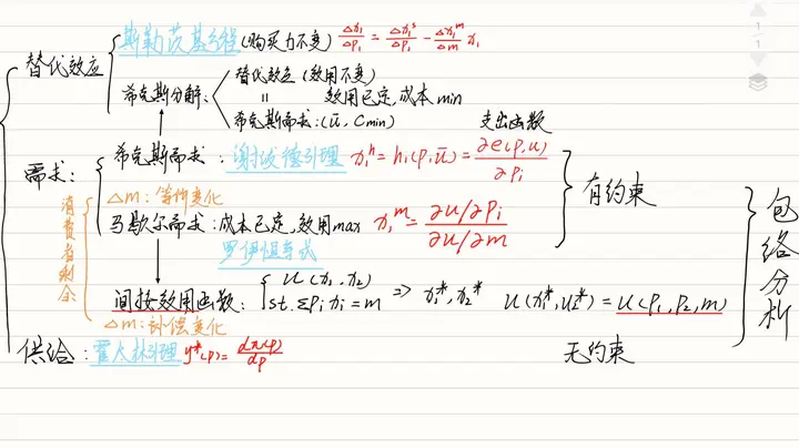
• Shepard’s lemma, given production functions, minimizes costs;
• Roy’s identity, given budget constraints, maximizes utility;
• Hotelling’s lemma is about unconstrained profit functions.

They are all analyses of envelope problems.

I. Shepard’s Lemma

Production Theory, Cost Minimization

Given the production function, minimize cost: $$ \min \sum_{i=1}^{n} w_i x_i \\ \text{subject to } \bar{y} = f(x_1, x_2, \ldots, x_n) $$

We construct the Lagrangian function to solve: $$ \mathcal{L} = \sum_{i=1}^{n} w_i x_i - \lambda (\bar{y} - f(x_1, x_2, \ldots, x_n)) $$

Taking partial derivatives with respect to $x_i$ and $\lambda$ and setting them to zero, we solve for the optimal input $x_i^*$ and substitute it into the cost function to obtain the minimum cost $\sum_{i=1}^{n} w_i x_i^*$.

Varian’s textbook often uses geometric methods: $$ \large \bbox[#def,10px,border: 5px solid]{\frac{\Delta x_2}{\Delta x_1} = -\frac{MP_1(x_1^*, x_2^*)}{MP_2(x_1^*, x_2^*)} = -\frac{w_1}{w_2}} $$

Proof Process:

$$ \begin{align} x_j(\mathbf{w}, y) &= \frac{\partial c(\mathbf{w}, y)}{\partial w_j} \\ &= \frac{\partial \sum_{i=1}^{n} w_i x_i}{\partial w_j} \\ &= x_j + \sum_{i=1}^{n} w_i \frac{\partial x_i}{\partial w_j} \end{align} $$

Given the first-order condition from the Lagrangian: $$ \frac{\partial \mathcal{L}}{\partial x_i} = w_i - \lambda f(x_1, \ldots, x_n) = 0 \\ \Rightarrow w_i = \lambda f(x_1, \ldots, x_n) $$

Substituting back, we get: $$ x_j + \lambda \sum_{i=1}^{n} f(x, \ldots, x) \frac{\partial x_i}{\partial w_j} $$

Given the production function constraint: $$ \bar{y} = f(x_1, x_2, \ldots, x_n) $$

Thus, the derivative with respect to $w_j$ is zero: $$ \frac{\partial \bar{y}}{\partial w_j} = \frac{\partial f(x_1, x_2, \ldots, x_n)}{\partial w_j} = 0 $$

Application Example:

Total cost function: $C = qv^{2/3}v^{1/3}$

(1) Use Shepard’s lemma to calculate the factor demand functions for kk and ll.

(2) Derive the potential production function based on the results from (1).

(1) $$ \begin{aligned} l &= \frac{\partial C}{\partial w} = \frac{2}{3} q \left(\frac{v}{w}\right)^{1/3} \\ k &= \frac{\partial C}{\partial v} = \frac{1}{3} q \left(\frac{w}{v}\right)^{2/3} \end{aligned} $$

(2) Eliminate $\frac{v}{w}$ from (1): $$ q = \left(\frac{3}{2}\right)^{2/3} 3^{1/3} l^{2/3} k^{1/3} = B l^{2/3} k^{1/3} $$ where $B = \left(\frac{3}{2}\right)^{2/3} 3^{1/3}$.

II. Roy’s Identity

Consumption Theory, Utility Maximization

Given budget constraints, maximize utility: $$ \max u = f(x_1, x_2, \ldots, x_n) \\ \text{subject to } \sum_{i=1}^{n} x_i p_i = m $$

Varian often uses geometric methods: $$ \large \bbox[#def,10px,border: 5px solid]{\frac{\Delta x_2}{\Delta x_1} = -\frac{MU_1(x_1^*, x_2^*)}{MU_2(x_1^*, x_2^*)} = -\frac{p_1}{p_2}} $$

Proof Process:

The Lagrangian function is: $$ \mathcal{L} = u(\mathbf{x}) - \lambda (\mathbf{p} \cdot \mathbf{x} - m) $$

Taking partial derivatives with respect to $x_i$: $$ \frac{\partial \mathcal{L}(\mathbf{x}^f, \lambda^f)}{\partial x_i} = \frac{\partial u(\mathbf{x}^f)}{\partial x_i} - \lambda^f p_i = 0 $$

The shadow price $\lambda$ is: $$ \lambda = \frac{\partial v(\mathbf{p}, m)}{\partial m} $$

Using Roy’s identity: $$ x_i^m = -\frac{\partial v / \partial p_i}{\partial v / \partial m} $$

Application Example:

Ping Xinqiao’s “Microeconomic Theory: Eighteen Lectures,” Lecture 16, “General Equilibrium and Two Fundamental Principles of Welfare Economics”

Given: $$ \begin{aligned} u^1(x_1, x_2) &= \min{x_1, x_2} & e^1 = (30, 0) \\ v^2(p, y) &= \frac{y}{2 \sqrt{p_1 p_2}} & e^2 = (0, 20) \end{aligned} $$

Find the Walrasian equilibrium.

III. Hotelling’s Lemma

Hotelling’s lemma is about unconstrained profit functions.

Production Theory, Profit Maximization

Given the profit function: $$ \pi(p) = \max_x p \cdot f(x(p, w)) - w \cdot x(p, w) $$

Hotelling’s lemma: $$ \large \bbox[#def,10px,border: 5px solid]{y^*(p) = \frac{d \pi(p)}{dp}} $$

Proof Process:

Given: $$ \pi(p) = \max_x p \cdot f(x(p, w)) - w \cdot x(p, w) $$

First-order condition: $$ p \frac{\partial f(x(p, w))}{\partial x} - w = 0 $$

Differentiating the profit function with respect to $p$: $$ \frac{\partial \pi(p, w)}{\partial p} = f(x(p, w)) + p \frac{d f(x(p, w))}{dx} \cdot \frac{\partial x(p, w)}{\partial p} - w \frac{\partial x(p, w)}{\partial p} $$

The blue part equals zero: $$ (p \frac{\partial f(x(p, w))}{\partial x} - w) \frac{\partial x(p, w)}{\partial p} = 0 $$

Application Example:

Ping Xinqiao’s “Microeconomic Theory: Eighteen Lectures,” Lecture 7, “Factor Demand Functions, Cost Functions, Profit Functions, and Supply Functions”

Given production function: $$ f(x_1, x_2) = 0.5 \ln x_1 + 0.5 \ln x_2 $$

Find the profit function $\pi(w_1, w_2, p)$ and derive the supply function using two methods.

IV. Supplement

These lemmas are based on envelope analysis in mathematical economics. The dual problems of cost minimization and profit maximization are dual problems, with parameters $\lambda$ being reciprocals.