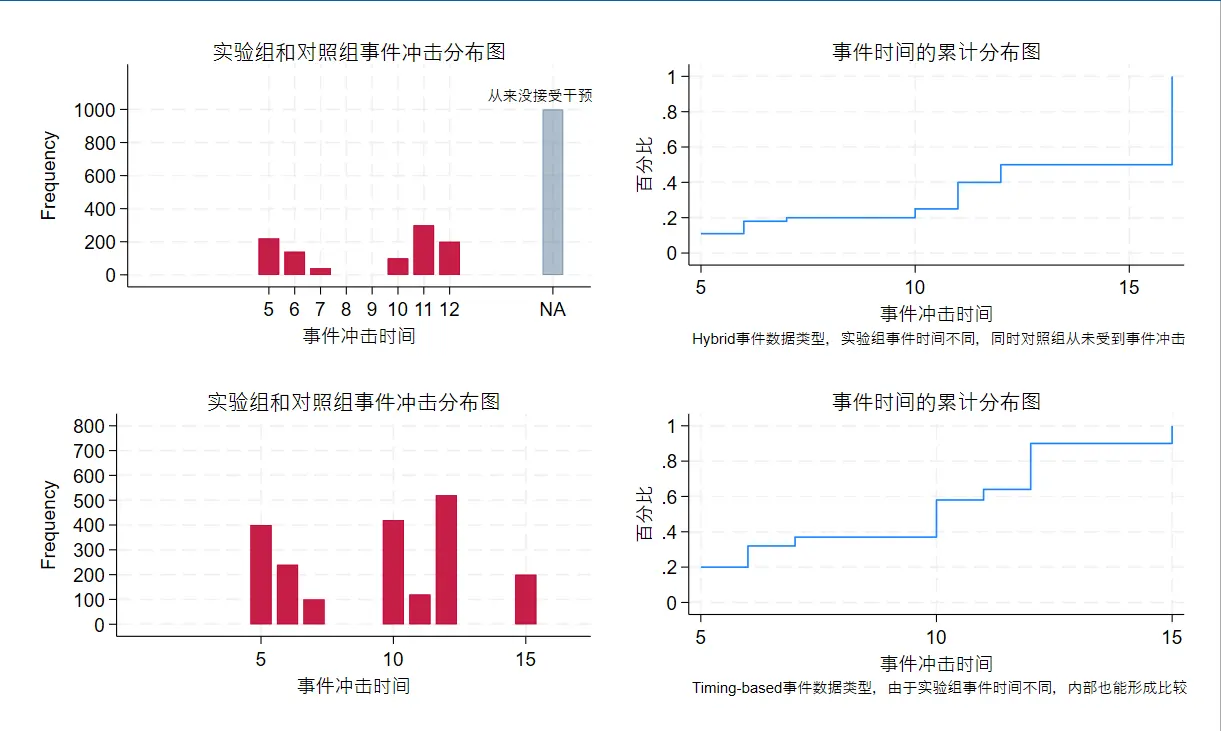
This code is descriptive statistics, describing the sample distribution (or serving as the background for policy implementation).
DID type: has both a treated group and a control group (which never received the policy)
Timing-based: only a treated group, but the event shock times differ within it.
Code output: the top row is a Hybrid data structure; the bottom row is a Timing-based data structure
The code below generates data, then draws a frequency plot and a cumulative plot. In the original, the cumulative plot first uses cumul to compute cumulative proportions and then uses twoway to draw a line chart. That’s too complicated, so here I’ve replaced it with the cdfplot command, which does it in one step.
Don’t be surprised if the result differs from the original — the original code also interpolates endpoint values on both sides, and I removed that part.
clear*-generaterandompaneldatafordifference-in-differencessetseed2024setobs100geni=_ngentreated=i>50genE_i=11iftreated==1expand20sortiquibyi:gent=_nxtsetit*-setthetreatmenteffectgenD=(t==E_i)genetime=(t-E_i)labelvari"个体编号"labelvart"日期"labelvarD"did变量=time*post"labelvarE_i"事件冲击时间"*-plotthedistributionofthetreatedandcontrolgroupsreplaceE_i=16iftreated==0replaceE_i=5iftreated==1&i>=51&i<=61replaceE_i=6iftreated==1&i>=62&i<=68replaceE_i=7iftreated==1&i>=69&i<=70replaceE_i=10iftreated==1&i>=71&i<=75replaceE_i=11iftreated==1&i>=76&i<=90replaceE_i=12iftreated==1&i>=91#delimit;/*
delimiter setting: change the semicolon to the line-break symbol for commands.
this way, unless a semicolon is added at the end, commands written across lines are read as one line.
this makes graphing commands much more convenient.
*/twoway(histogramE_iiftreated==1,discretefrequencystart(4)barwidth(0.8)xscale(range(017))yscale(range(01200))color(cranberry%100))(histogramE_iiftreated==0,discretefrequencystart(4)barwidth(0.8)xscale(range(017))yscale(range(01200))color(navy%40)),title("实验组和对照组事件冲击分布图",color(black)size(v.small))legend(off)xlabel(5"5"6"6"7"7"8"8"9"9"10"10"11"11"12"12"16"NA")text(110015.5"从来没接受干预",size(small))name(histogram4,replace);#delimitcr*-plotthedistributionofthetreatedandcontrolgroupspreserve//savethecurrentdataset#delimit;cdfplotE_i,title("事件时间的累计分布图",color(black)size(v.small))legend(off)ytitle(百分比)name(CDF4,replace)note(Hybrid事件数据类型,实验组事件时间不同,同时对照组从未受到事件冲击);#delimitcrrestore//reloadthesaveddataset*-distributionofthetreatedandcontrolgroupsreplacetreated=1replaceE_i=5iftreated==1&i>=1&i<=20replaceE_i=6iftreated==1&i>=21&i<=32replaceE_i=7iftreated==1&i>=33&i<=37replaceE_i=10iftreated==1&i>=38&i<=58replaceE_i=11iftreated==1&i>=59&i<=64replaceE_i=12iftreated==1&i>=65&i<=90replaceE_i=15iftreated==1&i>90#delimit;twoway(histogramE_iiftreated==1,discretefrequencystart(4)barwidth(0.8)xscale(range(017))yscale(range(0800))color(cranberry%100)),title("实验组和对照组事件冲击分布图",color(black)size(v.small))legend(off)ylabel(0(100)800)name(histogram5,replace);#delimitcr*-plotthecumulativedistributionofthetreatedandcontrolgroups#delimit;cdfplotE_i,title("事件时间的累计分布图",color(black)size(v.small))legend(off)ytitle(百分比)note(Timing-based事件数据类型,由于实验组事件时间不同,内部也能形成比较)name(CDF5,replace);#delimitcr*-combineanddisplaytheaboveplotsgraphcombinehistogram4CDF4histogram5CDF5iscale0.25//scaletheimagedowntoaquarter
Appendix B: Parameter restrictions for Timing-based
When estimating event effects in DID, you generally don’t add a time trend, but you do add individual fixed effects and time fixed effects, whose role is to decompose the intercept. The usual ways to handle collinearity are to default $t_{-1}$ to 0, merge or drop some variables, impose other constraints, or make it nonlinear……
For the Timing-based data form, since there is no control group, we can only compare within the treated group. More parameter restrictions are needed.
The variation in event timing is itself part of the information.
The larger the minimum difference in event timing across treated groups, the more information is lost.
The more individuals there are, the more information there is.
So what Appendix B’s code studies is —
When studying a Timing-based data structure, for different timing and individual distributions, how many additional parameters are needed to solve the problem?
My understanding: this may be a matter of building a system of equations through a series of regressions, forming a matrix from the system, and then judging via the matrix’s rank how many more parameter constraints are needed before it can be solved.
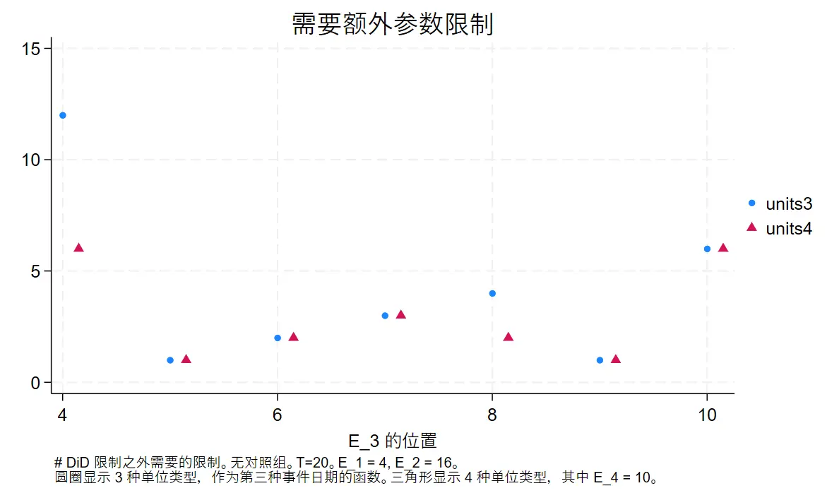
Appendix B code output: a figure the authors say is very strange
Let me explain what Appendix B’s output figure means.
First, take a dataset where everyone receives the event shock, but the event timing differs. In the initially generated dataset, the event shock times are 4 and 16. At this point the additional constraint parameters needed to solve are 12 (which can be understood as how many degrees of freedom are still missing).
Here’s what the figure means:
First look at the first column of blue dots.
When you add other samples whose event shock time is 4 (the x-axis), no extra information is added. The whole dataset is still two types of samples — event shock time 4 or 16 — so the additional parameters needed to solve are still 12 (the y-axis).
Similarly, the second column of blue dots means that when you add a third group of samples with shock time 5, the difference in event timing shrinks and information increases, so the additional parameters needed drop to 1.
The red triangles mean: on top of the dots in each column, what happens to the parameters needed when you add the samples the triangles represent.
I originally expected that, given a fixed timing difference, the more individual groups there are, the fewer additional parameters would be needed. It turns out only the fifth column behaves that way, which is why the paper says this is strange and worth studying — though the author doesn’t know why either.
#delimit;caplogclose;settraceoff;setmoreoff;clearall;setseed101;capprogdroprunme;progdefrunme;argslistctrltrends;quigendata"`list'"`ctrl' `trends';quiforvaluesi=0/20{;genD_p`i' = (etime == `i');//generatethepositivetreated-groupdummygenD_m`i' = (etime == -1 * `i');//generatethenegativetreated-groupdummysummD_p`i' ; // summarize the positive treated-group dummy
local dropme = (r(mean) == 0) ;
if `dropme'==1{;dropD_p`i' ; // if the mean is 0, drop the positive treated-group dummy
} ;
summ D_m`i';//summarizethenegativetreated-groupdummylocaldropme=(r(mean)==0);if`dropme' == 1 { ;
drop D_m`i';//ifthemeanis0,dropthenegativetreated-groupdummy};};dropD_m0;//dropthebaselinecaseofthenegativetreated-groupdummyegenunittype=group(E_i),miss;//generateaunit-typevariablefromE_i,handlingmissingvaluesquitabunittype,gen(udum);//summarizetheunit-typevariableandgeneratethecorrespondingdummiesquitabt,gen(tdum);//summarizethetimevariableandgeneratethecorrespondingdummiesunabvars:D_*udum*tdum*;//generatethevariablelistforeverythingrelatedtoD_*,udum*,andtdum*mata:count();//calltheMatafunctiontocomputevariablestatisticslocalc1=count[1,1];//getthefirstcolumnofthestatisticslocalc2=count[1,2];//getthesecondcolumnofthestatisticslocalc3=count[1,3];//getthethirdcolumnofthestatisticsdi"`list'"_column(20)`c1' _column(25) `c2'_column(35)`c3' ; // display the variable list and its statistics
end ;
mata: ;
void count()
{ ;
v = st_local("vars") ; // get the Stata local macro "vars"
X = st_data(.,v) ; // get the variable data from the current dataset
mycols = cols(X) ; // compute the number of columns of the data matrix
myrank = rank(X) ; // compute the number of non-missing values per column of the data matrix
gap = mycols - myrank ; // compute the number of missing values per column of the data matrix
output = (mycols,myrank,gap) ; // combine the statistics into a tuple
st_matrix("count",output) ; // store the statistics into a matrix named "count"
} ;
end ;
cap prog drop gendata ;
program define gendata ;
args list ctrl trends ;
drop _all ;
local numobs = 48 ; // define the number of observations
local treatedunittypes = wordcount("`list'") ; // compute the number of treated unit types
/* "ctrl" is 0/1 whether we have control (untreated) units */
/* if we have them, put half of data into control units */
local numtreatedobs = round(`numobs' / (1 + `ctrl')) ; // compute the number of treated-unit observations
local numuntreatedobs = `numobs' - `numtreatedobs' ; // compute the number of control-unit observations
local obspertype = floor(`numtreatedobs' /
`treatedunittypes') ; // compute the number of observations per treated unit type
forvalues i = 1/`treatedunittypes' { ;
local eventdate_`i' = word("`list'",`i');//gettheeventdateforeachtreatedunittype};setobs`numobs' ;/* number of observations */
gen i = _n ;
gen treated = i > `numuntreatedobs';/* treated-group units */genE_i=.;forvaluesi=1/`treatedunittypes' { ;
local start = (`i'-1)*`obspertype' + `numuntreatedobs'+1;localstop=(`i')*`obspertype'+`numuntreatedobs' ;
replace E_i = `eventdate_`i'' if i >= `start'&i<=`stop' ; // set the event date for each treated unit type
} ;
replace E_i = `eventdate_`treatedunittypes'' if i > `stop';tabE_i,miss;//summarizetheevent-datevariableandshowmissingvaluesexpand20;/* time span */sorti;quibyi:gent=_n;xtsetit;//definetheunitandtimevariablesforthepaneldata/* make variables that determine the DGP */genetime=(t-E_i);/* event time *//* gen TE = 1 * (etime >= 0) ;/* step-function treatment effect */
*/genTE=(etime>=0)*(etime+1);/* endless ramp-function treatment effect */replaceTE=0ifE_i==.;genY0_pure=0;/* the simplest counterfactual case */*genY0_pure=4*treated+0.3*treated*t;/* treated group has a pre-trend ... */*genY0_pure=4*treated+0.1*treated*(t-10)*(E_i-9);/* pre-trend based on E_i ... */geneps=sqrt(0.2)*rnormal();genactual=Y0_pure+TE*treated;geny=actual+eps;/* observed Y */end;capprogdropbigone;progdefbigone;runme"10 11"00;forvaluesi=4/16{;runme"4 16 `i' "00;localrest_m3_`i' = count[1,3] - 2 ;
runme "4 16 `i'10" 0 0 ;
local rest_m4_`i' = count[1,3] - 2 ;
} ;
drop _all ;
set obs 7 ;
gen E_i = _n + 3 ;
qui gen units3 = . ;
qui gen units4 = . ;
qui forvalues i = 4/10 { ;
replace units3 = `rest_m3_`i'' if E_i == `i' ;
replace units4 = `rest_m4_`i'' if E_i == `i' ;
} ;
gen E4_i = E_i + 0.15 ;
graph twoway (scatter units3 E_i , msymbol(o) msize(medsmall))
(scatter units4 E4_i , msymbol(triangle) msize(medsmall))
,
ti("需要额外参数限制")
xtitle("E_3的位置")
note("#DiD限制之外需要的限制。无对照组。T=20。E_1=4,E_2=16。"
"圆圈显示3种单位类型,作为第三种事件日期的函数。三角形显示4种单位类型,其中E_4=10。")
;
graph export figures/apdx_fig_A03.png , replace ;
end ;
bigone ;
So when we need additional constraints, how can we add them?
Method 3: not mentioned in the paper, but I have actually seen it used: $r1=2r_2$
These constrained regressions are implemented with the cnsreg command.
Appendix C: Choosing the estimator
There are currently two kinds of estimator choices:
Constrain the coefficient of the pre-event period variable to 0
Constrain the sum of the pre-event dummy variable coefficients to 0
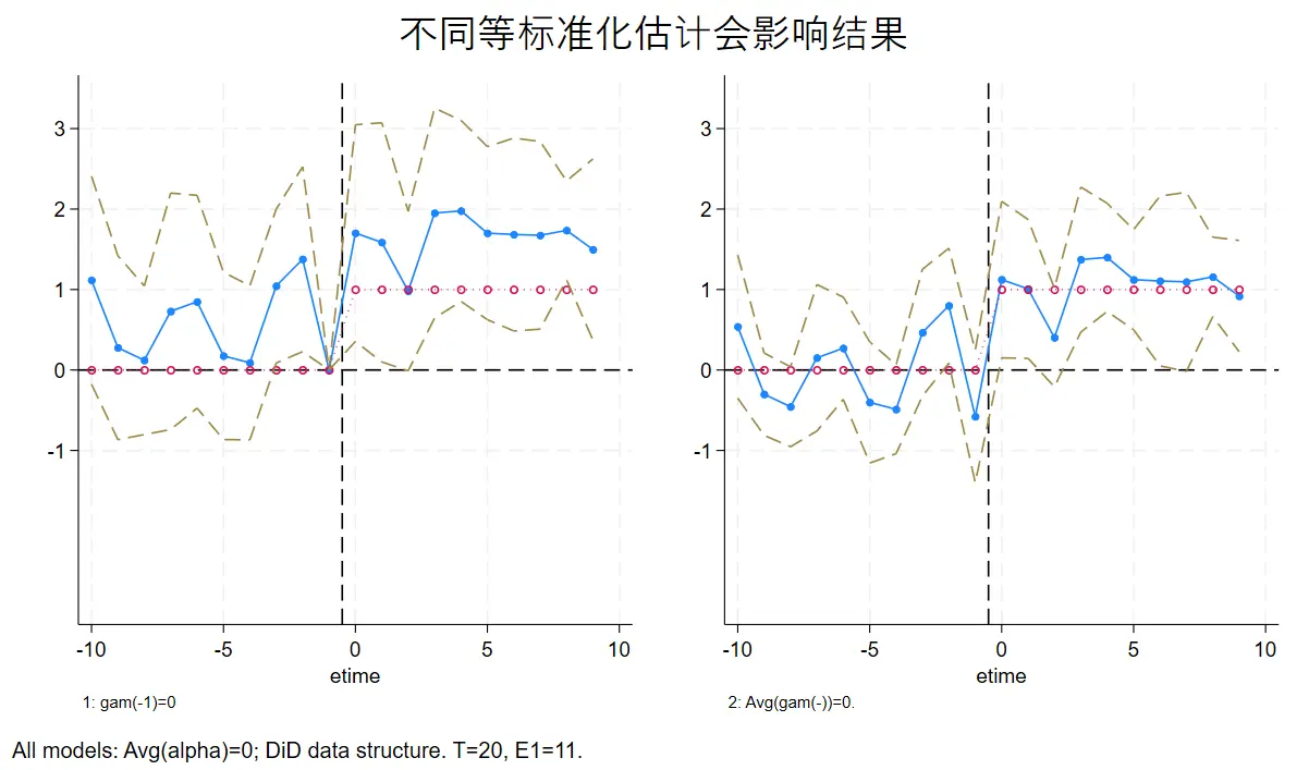
Estimation under different constraints; both estimators use individual fixed effects summing to 0The code in this part is a simulation experiment.
First, generate the treatment effect according to the conditions, with the treatment effect fixed at 1 (the red line in the figure is the actually generated treatment effect). Then add a random noise term, and finally run the regression.
The constraint on the left normalizes the pre-event period; the constraint on the right constrains the pre-event dummies. You can see the right one is closer to the actual treatment effect (the red line).
The following code has comments by GPT, with some corrections by me.
Code structure: define the data-structure generation function and the constraint-selection function, then plot.
#delimit;caplogclose;settraceoff;setmoreoff;clear;setseed2024202431;capprogdroprunme;progdefrunme;gendata;/* create the estimation variables *//* event-time dummies */forvaluesi=0/20{;genD_p`i' = (etime == `i');genD_m`i' = (etime == -1 * `i');summD_p`i' ;
local dropme = (r(mean) == 0) ;
if `dropme'==1{;dropD_p`i' ;
} ;
summ D_m`i';localdropme=(r(mean)==0);if`dropme' == 1 { ;
drop D_m`i';};};dropD_m0;genbytegroup2=E_i==11;gentrend_group2=t*group2;summ;/* 1 normalize the event-time dummy at -1 to 0 */constraintdefine1D_m1=0;/* 2, the fixed effects of all groups sum to 0 */constraintdefine21.i+2.i+3.i+4.i+5.i+6.i+7.i+8.i+9.i+10.i=0;/* 7 set the average of the pre-treatment event-time dummies to zero*/constraintdefine7D_m10+D_m9+D_m8+D_m7+D_m6+D_m5+D_m4+D_m3+D_m2+D_m1=0;cnsregyD_m*D_p*ibn.tibn.i,cluster(i)noconsconstraints(21)collinear;matrixmyb_ES1=e(b);matrixmyV_ES1=e(V);cnsregyD_m*D_p*ibn.tibn.i,cluster(i)noconsconstraints(27)collinear;matrixmyb_ES2=e(b);matrixmyV_ES2=e(V);tempfilemain;save`main' ;
/* plot */
*start debugging;
tempfile pooled ;
forvalues i = 0/10 { ;
drop _all ;
set obs 2 ;
gen label = "m`i'" in 1 ;
replace label = "p`i'" in 2 ;
gen etime = -1 * `i'in1;replaceetime=`i' in 2 ;
foreach j in 1 2 { ;
gen cf_m`j'=.;/* set the estimation equation for the treatment effect */gentruth_m`j' = (0) in 1 ;
replace truth_m`j'=(1)in2;localmyb=0;caplocalmyb=myb_ES`j'[1,"D_m`i'"] ;
gen ES_b_m`j' = `myb' in 1 ;
local myv = . ;
cap local myv = myV_ES`j'["D_m`i'","D_m`i'"] ;
local myse = sqrt(`myv') ;
gen ES_se_m`j' = `myse' in 1 ;
local myb = 0 ;
cap local myb = myb_ES`j'[1,"D_p`i'"] ;
replace ES_b_m`j'=`myb' in 2 ;
local myv = . ;
cap local myv = myV_ES`j'["D_p`i'","D_p`i'"];localmyse=sqrt(`myv') ;
replace ES_se_m`j'=`myse' in 2 ;
} ;
capture append using `pooled';save`pooled' , replace ;
} ;
drop if label == "m0" ;
drop if label == "p10" ;
sort etime ;
save `pooled',replace;localnote1"gam(-1)=0";localnote2"Avg(gam(-))=0.";forvaluesi=1/2{;gentop_`i' = ES_b_m`i'+1.96*ES_se_m`i' ;
gen bot_`i'=ES_b_m`i' - 1.96 * ES_se_m`i';graphtwoway(connectedES_b_m`i' truth_m`i'etime,msize(medsmallmedium)msymbol(ooh)lpattern(soliddot))(linecf_m`i' etime , lpattern(dash) )
(line top_`i'bot_`i' etime, lpattern(dash dash) lcolor(brown brown))
, legend(off) xline(-0.5)
note("`i':`note`i''")
name(g`i' , replace) yscale(range(-3,3.5)) yline(0 , lpattern(dash) lcolor(black)) ;
} ;
graph combine g1 g2 , ti("不同等标准化估计会影响结果")
note("Allmodels:Avg(alpha)=0;DiDdatastructure.T=20,E1=11.") ;
graph export figures/apdx_fig_A04.png , replace ;
end ;
cap prog drop gendata ;
program define gendata ;
/*****************
main data-generation process options
/* possible treatment-effect types */
1 - zero treatment effect
2 - step-function treatment effect
3 - permanent ramp
4 - ramp to plateau
5 - AR(1) type
/* distribution of E_i */
T = 19; E_i ~ U(6,14)
/* are there never-treated units? */
yes; no
/* Y0 (the "signal" of the potential outcome) dynamics */
1 - baseline: Y0 = 0
2 - level shift: Y0_i,t = E_i
3 - trend shift: Y0_i,t = t * E_i
end of main options
******************/
drop _all ;
/*
/* classic ES data structure */
set obs 9 ;/* number of groups */
gen i = _n ;
gen E_i = 5 + i ;
gen treated = 1 ;/* all treated */
expand 20 ;/* number of periods */
*/
set obs 10 ;/* number of groups */
gen i = _n ;
/* NxT DiD data structure*/
gen treated = i > 5 ;/* half treated */
gen E_i = 11 if treated == 1 ;
expand 20 ;/* number of periods */
sort i ;
qui by i: gen t = _n ;
xtset i t ;
/* create variables that determine the DGP */
gen D = (t == E_i) ; /* the event "pulse" */
gen etime = (t - E_i) ;/* event-time dummy */
gen TE = 1 * (etime >= 0) ;/* treated-group indicator */
*gen TE = (etime >= 0) * (etime+1) ;/* endless ramp function for treatment effect */
replace TE = 0 if E_i == . ;
gen treated_post = etime >= 0 ;
gen Y0_pure = 0 + 1 * treated ;/* offset counterfactual */
*gen Y0_pure = 4 * treated + 0.3 * treated * t ;/* treated have a pre-trend ... */
*gen Y0_pure = 4 * treated + 0.01 * treated * (t-10) * (E_i - 9);/* pre-trend based on E_i ... */
gen eps = sqrt(0.3) * rnormal() ;
gen actual = Y0_pure + TE * treated ;
gen y = actual + eps ;/* observed Y */
end ;
runme ;
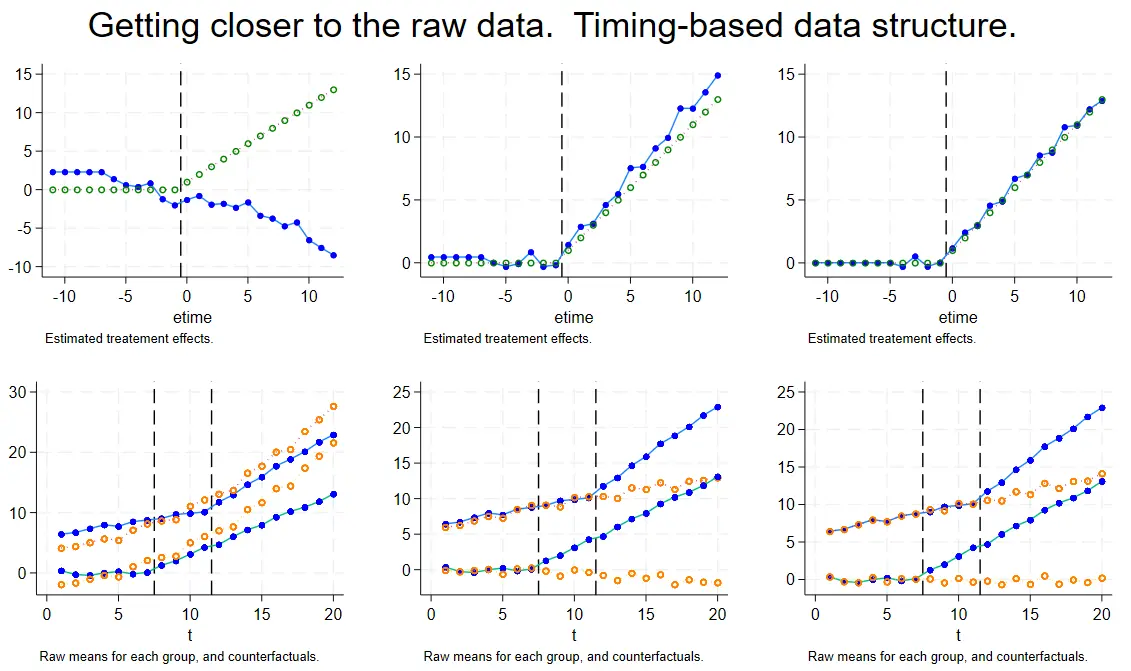
The rest of part C is a Timing-based data simulation; the code structure is the same, only the data structure and constraints differ, so I won’t repeat it here — I’ll just show the output.
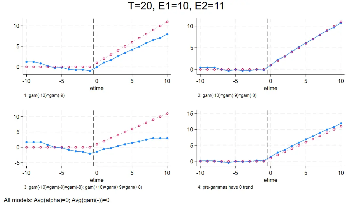
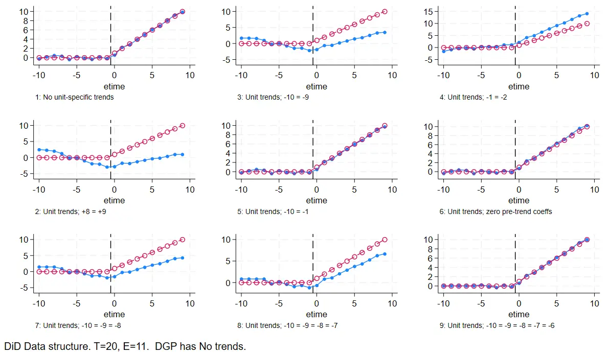
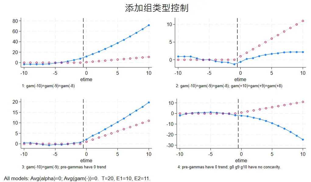
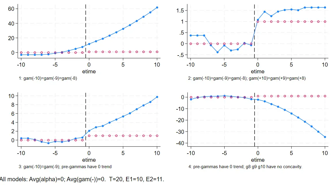
Timing-based structure data
Top-left: only the first two time-dummy coefficients are constrained to be equal.
Top-right: the first three time-dummy coefficients are constrained to be equal.
Bottom-left: the three periods on each side of pre/post are constrained to have equal coefficients.
Bottom-right: the pre-event anticipatory-effect dummy coefficients are constrained to sum to 0.
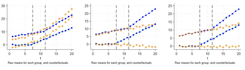
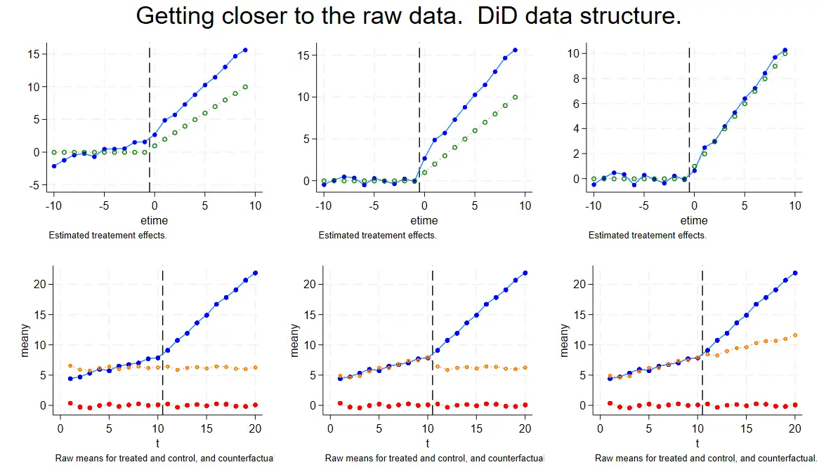
Appendix D can essentially be understood as a decomposition that adds a time trend (a slope comparison). The code structure is the same as before; what’s added this time is predicting the counterfactual group, and using it to strengthen the causal argument through another comparison.
/* create the counterfactual prediction cf_ES2 */gencf_ES2=y;//initializecf_ES2astheobservedvariabley/* loop over the time range */quisummetime;//getsummarystatisticsofetimelocalmymin=r(min);//gettheminimumlocalmymax=r(max);//getthemaximumforvaluesi=`mymin'/`mymax'{//loopoverthetimerangeif`i' < 0 { // if time is less than 0
local j = abs(`i');//taketheabsolutevaluereplacecf_ES2=cf_ES2-_b[D_m`j'] * D_m`j';//subtractthetreatment-effectcoefficienttimesthecorrespondingdummy}else{//iftimeisgreaterthanorequalto0replacecf_ES2=cf_ES2-_b[D_p`i'] * D_p`i';//subtractthetreatment-effectcoefficienttimesthecorrespondingdummy}}/* compute the counterfactual prediction mean by unit type and time */egenmeancf_ES2=mean(cf_ES2),by(tunittype);//computethemeanofcf_ES2bytandunittype
Taking the difference of the coefficients before and after use again to get the result
Appendix E: Repeated event shocks
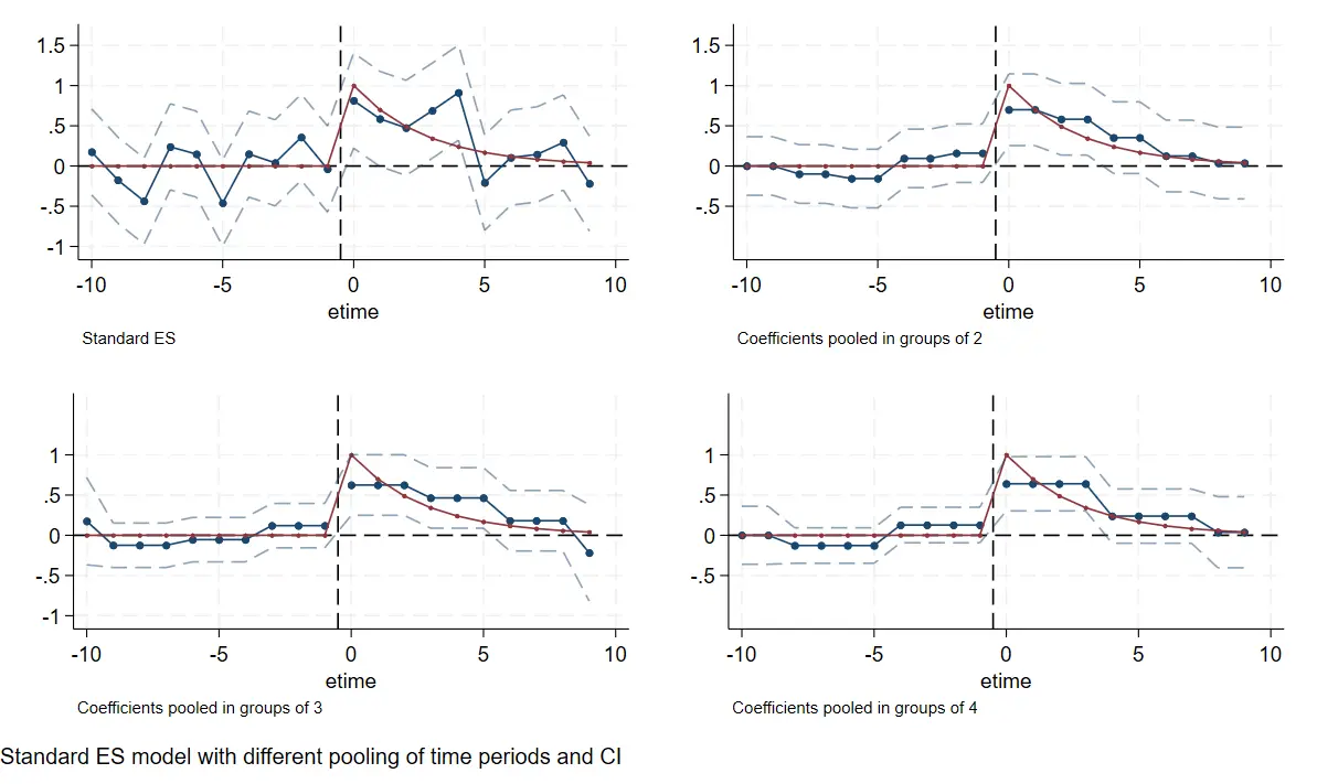
The problem this part solves is: if an event occurs repeatedly at different times, how should you choose? Here the generated true treatment effect is a continuously decaying curve.
Approach 1 constrains the coefficients of the event dummies to be equal ($\gamma_1=\gamma_2$):
The constraints below are segmentations into two-period, three-period, and four-period groups.
#delimit;/*two periods per group*/constraintdefine9D_m10=D_m9;constraintdefine10D_m8=D_m7;constraintdefine11D_m6=D_m5;constraintdefine12D_m4=D_m3;constraintdefine13D_m2=D_m1;constraintdefine14D_p0=D_p1;constraintdefine15D_p2=D_p3;constraintdefine16D_p4=D_p5;constraintdefine17D_p6=D_p7;constraintdefine18D_p8=D_p9;/*three periods per group */#delimit;constraintdefine21D_m1=D_m2;constraintdefine22D_m1=D_m3;constraintdefine23D_m4=D_m5;constraintdefine24D_m4=D_m6;constraintdefine25D_m7=D_m8;constraintdefine26D_m7=D_m9;constraintdefine27D_p0=D_p1;constraintdefine28D_p2=D_p1;constraintdefine29D_p3=D_p4;constraintdefine30D_p3=D_p5;constraintdefine31D_p6=D_p7;constraintdefine32D_p6=D_p8;
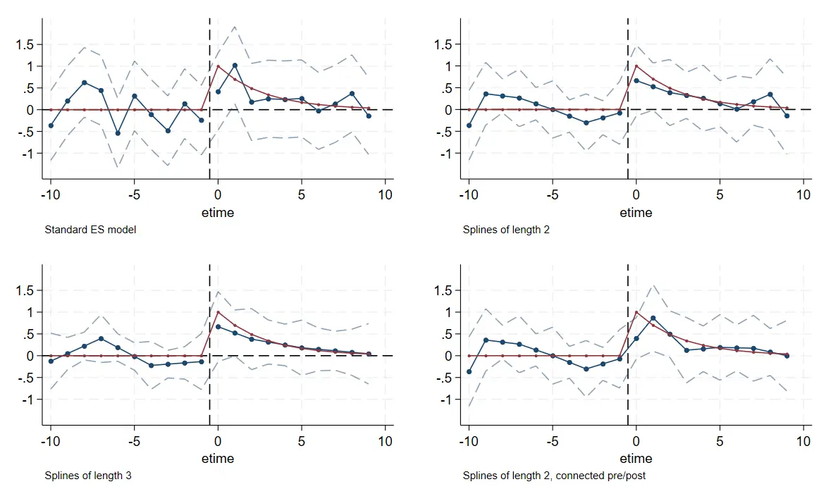
Approach one: constrain the event-time dummy values to be equalApproach 2 constrains the slopes between coefficients to be equal ($\gamma_1-\gamma_0=\gamma_2-\gamma_1$)
The constraints applied include the trend control and the event-time dummy constraints
Time-based: one unit, two times
Next, verify the Time-based data form.
The DID form has a control group to help generate counterfactual predictions, but time-based lacks a control group. The usual options are:
The event-time dummy coefficients for the earliest and latest periods are equal, making the plot smoother
The slopes between the earliest and latest event-time dummy coefficients are equal, better showing the trend
The sum of the pre-trend coefficients is constrained to 0
The trend-weighted constraints across multiple event times sum to 0
You can see that in the experiment below, the fourth plot actually produced a strange result.
The constraints applied were:
Individual fixed effects sum to 0
Pre-event effects sum to 0
The slopes at the end of the post-event period are equal
The weighted pre-trend is 0
1
2
3
4
\\Idon't understand where the 5.5 base period in this constraint comes from?
constraint define 8 (10-5.5)*D_m10 + (9-5.5)*D_m9 + (8-5.5)*D_m8 + (7-5.5)*D_m7
+ (6-5.5)*D_m6 + (5-5.5)*D_m5 + (4-5.5)*D_m4 +
(3-5.5)*D_m3 + (2-5.5)*D_m2 + (1-5.5)*D_m1 = 0 ;
time-based simulation
So should we choose the constraint that the coefficients’ slopes are equal or that the coefficient values are equal?
The answer depends on the situation. If a policy’s true effect doesn’t change over time, choose the equal coefficient values constraint; if the policy effect changes over time, choose the equal coefficient slopes constraint.Simulation of a jump shock whose effect doesn’t change over time, where the equal-coefficient-values estimator is more efficient
I think this conclusion has become circular reasoning. The whole point of event studies is to estimate the treatment effect (whether it is dynamic or static is precisely what we need to find out), and now it’s turned into choosing the method based on the result.
Still, the takeaway is simply to analyze the policy background, form an assumption, and then choose the constraint.
DID: many units, many times
For multi-period DID, adding multiple event-time trend-weighted constraints that sum to 0 makes the estimation more efficient. As shown:
The first column is the ordinary estimate, with no restrictions beyond two-way individual and time fixed effects.
The second column adds, on top of the first, the constraint that the pre-event trends sum to 0:
1
2
3
4
//eventdatesarestill10and5;Idon't understand where the 5.5 base period comes from
constraint define 3 -4.5*D_m10 - 3.5*D_m9 - 2.5* D_m8 - 1.5* D_m7
- 0.5*D_m6 + 0.5 * D_m5 + 1.5 * D_m4 +
2.5 *D_m3 + 3.5 *D_m2 + 4.5 *D_m1 = 0 ;
The third column adds a type control:
1
gentreated_time=treated*t
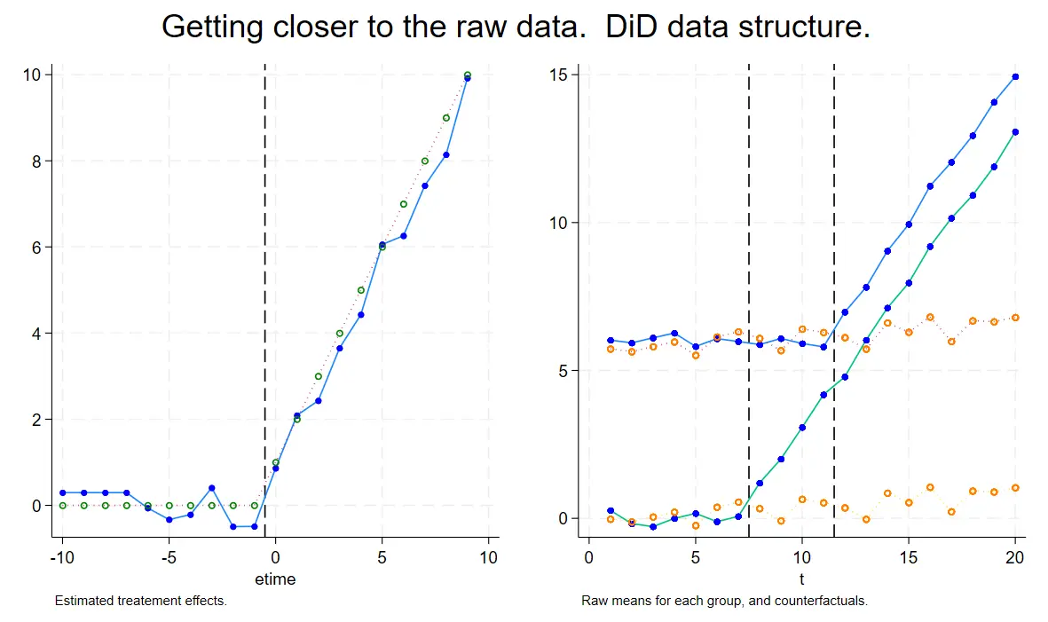
DID estimation: the orange part is the counterfactual group predicted from residuals
Time-based: many units, many times
time-based; orange is also the counterfactual groupAbove is a Time-based structure where everything is the treated group, but this time there are individual differences.
The second column adds, on top of the first, individual grouping and a time-weighted trend of 0:
1
2
3
4
5
6
//individualgroupingEgenunittype=group(E_i);Egenmeany=mean(y),by(tunittype)//time-trendweighting;Istilldon't understand where the 3.5 base period comes from
constraint define 103 (6-3.5) * D_m6 + (5-3.5) * D_m5 +
(4-3.5) * D_m4 + (3-3.5) * D_m3 + (2-3.5) * D_m2 + (1-3.5) * D_m1 = 0 ;
The third column adds coefficient constraints on top of the second:
My understanding is that event studies further slice DID over time. Because there are more time dummies, solving requires more constraints, so we have to add time-trend controls based on the research context.
DID and event studies complement each other; event studies can further show the dynamic effects of the DID estimate (increasing, decreasing, or reverting to the normal value after variation over time). If the two estimates point in opposite directions, it may be because the wrong constraints were chosen, or there is a collinearity issue.
Different data structures call for different numbers and types of additional constraints in event studies.
From the appendix-code experiments —
Solving a Time-based dataset requires adding constraints, and how many depends on the number of event times and individuals.
In event studies, standardizing the pre-trend generally tends to be more accurate.
A dataset with only one unit but shocks at different times needs constraints added carefully, or you may get the opposite result.
Data with many individuals, whether time-based or did, should add a group-type control.

 滑翔闪 included in Economic Studies and Event Studies