HLT: Lifecycle and Wage Decomposition

APC panel and life cycle

The Mincer earnings function , which was discussed earlier, examines the relationship between returns on human capital investment. ¹

$$ ln(w)=\alpha_0+\beta_ss+\beta_0\exp+\beta_1\exp^2+\gamma X_i+\varepsilon$$

$s$ represents the level of education, $exp$ represents the level of work experience, and $X_i$ denotes other control variables.

Here, it is assumed that the returns to education are linear and the returns to work experience are nonlinear for the logarithmized wages. Heckman et al. (2006) empirically tested this assumption in their related research ².

Even if we don’t discuss the specific form of the equation, such a decomposition of variables is certainly insufficient.

As the famous bread hunter DIO once said——

“JOJO, in the brief span of a human life, I have discovered… The more one plays with schemes, the more limited one finds the capabilities of humanity to be…” Indeed! Human lifespan and physical stages are points we cannot ignore! Once we delve into labor economics, we cannot avoid discussing human age and condition.

Firstly, let’s consider the lifecycle. Even if individuals have the same education level and work experience, or even higher, the rate of return on education varies with age. Here, we estimate parameters that are age and time-related. Moreover, the historical context in which each individual exists also influences wage earnings. For instance, movements like “going to the countryside” and “reform and opening up” deeply affected specific cohorts. Here, we estimate parameters (usually categorized by birth year) that are related to individual cohorts and time. Additionally, time effects (including economic cycles and linear growth, such as wage inflation) are also related to time! All these parameters are time-dependent! Decomposing them in the econometric equation becomes a significant challenge. Hence, we have the following extended and flexible Mincer equation.

$$ln(w_{ict})=\alpha+\theta(s_{ict})+f(x_{ict})+\gamma_{t}+\chi_{c}+\varepsilon_{ict}$$

$i$ represents an independent number. $c$ represents the group number, for example, one group was born during the reform and opening up, one group was born when people went to the mountains and countryside, and one cohort group ³. In the life cycle, work experience is generally divided into groups. The descriptive statistics in the figure below are preliminary descriptive statistics of the life cycle carried out by comparing groups after five years of grouping. $t$ represents the time variable. $\theta(s_{ict})$ represents the education income function, $f(x_{ict})$ represents the work experience income function, $\gamma_t$ represents the queue effect of group $c$, $\chi_t$ represents the group queue Effect, $\varepsilon_{ict}$ is the paper.

Individual-level panel data is often challenging to obtain directly. Therefore, Deaton proposed:

“We don’t need individual tracking panels anymore! Your room has no space left for you to obtain positions! We’ll synthesize a ‘pseudo-panel’ from repeated cross-sections of census data! Epidemiology, drug trials, social psychology, and other statistical fields all make use of such pseudo-panels.

For example, in the figure below: These income comparison data are not from individual tracking panel data but rather from a pseudo-panel constructed from cross-sectional data of different ages at the same time.”

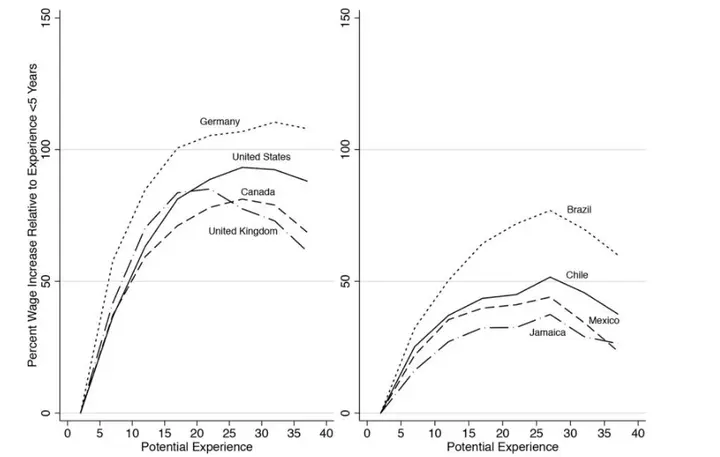
This type of panel data requires consideration of age, time period, and cohort as independent variables, also known as the Age-Period-Cohort Model (APC). In labor economics, the estimation of APC panel data has always been a hot topic (endorsed by the great Deaton, after all, it is a framework he established in economic analysis).

For the estimation equation:

$$ln(w_{ict})=\alpha+\theta(s_{ict})+f(x_{ict})+\gamma_{t}+\chi_{c}+\varepsilon_{ict}$$

When we directly regress APC data, we encounter the problem of collinearity—age + birth year = current year.

Deaton’s approach（mathematical Decomposition）

Angus Deaton, who won the Nobel Prize in 2015 for his research on poverty, has made significant contributions to labor economics, with much discussion focused on his findings that aid may worsen conditions ⁴.

The following method is mainly based on his work “The Analysis of Household Surveys: A Microeconometric Approach to Development Policy” (1997) (starting from page 123), to be honest, it feels a bit, well, unfriendly.

For the formula:

$$ln(w_{ict})=\alpha+\theta(s_{ict})+f(x_{ict})+\gamma_{t}+\chi_{c}+\varepsilon_{ict}$$

Like this:

$$w_{ict}=\exp (\alpha+\theta(s_{ict})+f(x_{ict})+\gamma_{t}+\chi_{c}+\varepsilon_{ict})$$

The aggregate total wage can be decomposed into sums grouped first by $c$, and within each group, summed over individuals $i$:

$$\begin{aligned} \sum_{i=1}^{N_{ct}}w_{ict}=& \sum_{i=1}^{N_{ct}}\exp(\alpha+\theta(s_{ict})+f(x_{ict})+\gamma_{t}+\chi_{c}+\varepsilon_{ict}) \newline &=\exp(\alpha+\gamma_t+\chi_c)\underbrace{\sum_{i=1}^{N_{ct}}\exp(\theta(s_{ict})+f(x_{ict})+\varepsilon_{ict})}_{F_{ct}} \newline &=\exp(\alpha+\gamma_{t}+\chi_{c})F_{ct} \end{aligned}$$

$F_{ct}$ at this point represents the total wage contribution of both the education experience function $\theta(s_{ict})$ and the work experience function $f(x_{ict})$.

Define $\bar{F}_t = \sum*{c\in C_t} F_{ct}$, then proceed to separate this part out, transforming it as follows:

$$\begin{aligned} W_{t}=& \sum_{c\in C_{t}}\sum_{i=1}^{N_{ct}}w_{ict} \newline &=\sum_{c\in C_{t}}\exp(\alpha+\gamma_{t}+\chi_{c})F_{ct} \newline &=\exp(\alpha)\exp(\gamma_{t})\sum_{c\in C_{t}}\exp(\chi_{c})F_{ct} \newline &=\exp(\alpha)\exp(\gamma_{t})\bar{F}_{t}\sum_{c\in C_{t}}\exp(\chi_{c})\frac{F_{ct}}{\bar{F}_{t}} \end{aligned}$$

At this point, wages can be decomposed into three parts: time effect $\Gamma_{t}$, the effect of work experience and education $\bar F_{t}$, and cohort effect $\bar X_{t}$.

$$W_{t}=\underbrace{\exp(\gamma_{t})}_{\Gamma_{t}}\bar F_{t}\underbrace{\sum_{c\in C_{t}}\exp(\chi_{c})\frac{F_{ct}}{\overline{F_{t}}}}_{\tilde{X_{t}}}$$

The effects of work experience and education can be quantified through the years of education and work, but identifying the time effect and cohort effect is challenging. Therefore, the purpose of this approach is to isolate and study the time and cohort effects separately. Hence, we define:

$$\Omega_{t}=\frac{W_t}{\bar F_{t}}=\Gamma_{t}\bar{X}_{t}$$

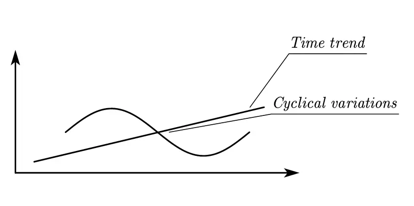
In studying cohort and time effects, we typically approach it from two perspectives.

• Time trend: Our technology always advances over time, representing a time trend that progresses on average.
• Cyclical variations: For example, seasonal vegetables have cyclical supply and demand patterns, or the baby boom generation—when the baby boomers reach middle age, there may be a peak in the labor force.

At the same time, it should be emphasized that what is defined is that $\bar{\chi}_t$ and $\bar{\gamma}_t$ are the deviations of the sample mean at this time. Just like we assume that the sum of residuals after regression is 0, this assumption also requires that the sum of sample mean residuals is 0:

$$\frac1T\sum_{t=0}^T\gamma_t=\frac1T\sum_{t=0}^T\bar{\chi}_t=0$$

At this time, the formula is decomposed into: $\omega_t=\bar{\omega}+\bar \gamma_t+\bar{\chi}_t$

The original paper only stated that $\bar{\omega}$ is “an appropriately chosen constant”. Personally, I think it is the sample mean, so in contrast, $\bar{\chi}_t$ and ${\bar \gamma}_t$ are the deviations from the sample mean.

At this time, both the time effect and the queue effect can be decomposed into time trend$g$ and periodic change $u$, which can be expressed by $gt+u$, and the following decomposition is obtained:

$$\gamma_{t}=g_{\gamma}t+u_{\gamma,t},\quad\bar{\chi}_{t}=g_{\bar \chi}t+u_{\bar \chi,t}$$

We make $g_{\omega}=g_{\bar \gamma}+g_{\bar{\chi}}$, and the final estimate becomes $$\omega_t=\bar{w} _t+g_\omega t+u_{\omega,t}$$

Deaton (1997) ⁵ is unable to do anything at this point. He can only perform enumeration processing.

• The residual decomposition is all explained as time effects: $g_{\omega}=g_{\bar \gamma}+g_{\bar{\chi}}=g_{\bar \gamma}$
• The residual decomposition is all explained as cohort effects: $g_{\omega}=g_{\bar \gamma}+g_{\bar{\chi}}=g_{\bar{\chi}}$
• You two are evenly divided, each gets half: $\frac{1}{2}g_{\omega}=g_{\bar \gamma}=g_{\bar{\chi}}$

Quantitative decomposition

That is to say, the following formula is estimated:

$$\log(w_{ict})=\alpha+\theta(s_{ict})+\sum_{x\in\mathbf{X}}\phi_{x}D_{ict}^{x}+\gamma_ {t}+\chi_{c}+\varepsilon_{ict}$$

$\theta(s_{ict})$ represents the income function of educational age, which is generally expressed linearly.

$D_{ict}^{x}$ is a dummy variable for each age group in the life cycle.

$\gamma_{t}$: time effect. $\chi_{c}$ individual effects.

Directly use this formula to regression, $D_{ict}^{x}$, $\gamma_{t}$, $\chi_{c}$ have collinearity, the Deaton method is to give $\gamma_{t}$, $\chi_{c}$ imposes an additional linear constraint. When we set only the queue effect and the time effect to 0, we need to satisfy $\sum_{t=0}^{T}\gamma_{t}t=0$. We can achieve this by “normalizing” $\gamma_{t}$:

Definition

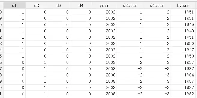
$$\quad d_t^*=d_t-[(t-1)d_2-(t-2)d_1]$$

$t$ is the year label. When this data is in year $t$, it is 1, otherwise it is 0. The corresponding stata operation is

1

tab year ,gen(d)

For example,

High-order difference method estimation

Deaton estimated that the year and cohort effects were actually a bit extreme, either taking them all or dividing them equally, and were criticized by later generations as having “no theoretical basis.” Some scholars have suggested that we cannot find the growth rate (first-order derivative), so we can use high-order differences to estimate the second-order and above, so that we can verify the general shape of the year and group effects!

If you want to see the super-detailed derivation, it is recommended to check out “Disentangling age, cohort and time effects in the additive model” (McKenzie et al., 2006) ⁶.

1

For the estimated formula:

$$ ln(w_{ict})=\alpha+\theta(s_{ict})+f(x_{ict})+\gamma_{t}+\chi_{c}+\varepsilon_{ict} $$ Direct regression will have the problem of collinearity - age + year of birth = current year. We cannot directly estimate the form of $\gamma_t$ and $\chi_t$ (such as concavity and convexity), but we can use the difference method to study the properties of high-order differences after group subtraction, and then estimate low-order differences.

In the life cycle model here, the years of education are linear estimates and easy to decompose, so we ignore ⁷ for now. The individual number is $i$, and the queue is grouped $c$ according to the life cycle. $k$ is the work experience, which is equal to $t-c$. The corresponding equations for each group of queues are as follows: $$ y_{ct}=\alpha+\beta _kx_{ct}+\gamma_{t}+\chi_{c}+\varepsilon_{ct} $$

**Emphasis! In other words, the estimate of $\color{red}{k}$ of $\beta_{\color{red}{k}}$ is closely related to $\color{blue}{k=t-c}$! ! ! ! We take advantage of this to perform high-order difference estimation. **

We are in the same group (for example, we select the middle-aged group $c_1$), and use the data of $y_{c_1,t_2}$ minus $y_{c_1,t_1}$ to carry out the time analysis within the group. The first difference** of:

During the life cycle, the time difference of each group of queues is evenly distributed, basically every five years, that is $$ (x_{ci,t+1}-x_{ci,t})=(x_{cj,t+1}-x_{cj,t})=\Delta x_t $$ So the formula can be transformed as follows: $$ \begin{align} &y_{c_1,t_2}-y_{c_1,t_1}\newline &=(\beta_{\color{red}{k_{2}}}- \beta_{\color{red}{k_{1}}})(x_{c_1,t_2}- x_{c_1,t_1})+(\gamma_{t_2}-\gamma_{t_1})+(\varepsilon_{c_1,t_2}-\varepsilon_{c_1,t_1})\newline &=(\beta_{\color{red}{k_{2}}}- \beta_{\color{red}{k_{1}}})\Delta x_t+(\gamma_{t_2}-\gamma_{t_1})+(\varepsilon_{c_1,t_2}-\varepsilon_{c_1,t_1})\newline \end{align} $$ The corresponding time relationship $k=t-c$, we then perform the first-order difference in time on another same group.

We select a group $c_{0}$ that is younger than group $c_{1}$ (regarded as a youth group), and get $k_2=t_1-c_0,k_3=t_2-c_0$.

At this point the first difference is obtained: $$ \begin{align} &y_{c_0,t_2}-y_{c_0,t_1}\newline &=(\beta_{\color{red}{k_{3}}}- \beta_{\color{red}{k_{2}}})\Delta x_t+(\gamma_{t_1+1}-\gamma_{t_1})+(\varepsilon_{c_0,t_2}-\varepsilon_{c_0,t_1})\newline \end{align} $$ At this time, we subtract the first-order differences of $c_1$ and $c_0$ the two sets of time: $$ \begin{align} &[y_{c_1,t_2}-y_{c_1,t_1}]-[y_{c_0,t_2}-y_{c_0,t_1}]\newline &=(\beta_{\color{red}{k_{2}}}- \beta_{\color{red}{k_{1}}})\Delta x_t+(\gamma_{t_1+1}-\gamma_{t_1})+(\varepsilon_{c_1,t_2}-\varepsilon_{c_1,t_1})\newline &-(\beta_{\color{red}{k_{3}}}- \beta_{\color{red}{k_{2}}})\Delta x_t-(\gamma_{t_1+1}-\gamma_{t_1})-(\varepsilon_{c_0,t_2}-\varepsilon_{c_0,t_1})\newline &=[(\beta_{\color{red}{k_{2}}}- \beta_{\color{red}{k_{1}}})-(\beta_{\color{red}{k_{3}}}- \beta_{\color{red}{k_{2}}})]\Delta x_t-\Delta_{c}\Delta_{t}\varepsilon_{c_{0},t_{2}} \end{align} $$ We can find that this high-order difference does not contain time effect $\gamma_t$ and queue effect $\chi_c$ at this time.

$[(\beta_{\color{red}{k_{j}}}- \beta_{\color{red}{k_{j-1}}})-(\beta_{\color{red}{k_{ j+2}}}- \beta_{\color{red}{k_{j}}})]$ also has geometric meaning. For the formula: $$ y_{ct}=\alpha+\beta _kx_{ct}+\gamma_{t}+\chi_{c}+\varepsilon_{ct} $$ $[(\beta_{\color{red}{k_{j}}}- \beta_{\color{red}{k_{j-1}}})-(\beta_{\color{red}{k_{ j+2}}}- \beta_{\color{red}{k_{j}}})]$ is the slope of $\beta _k$. It is similar to the situation where we cannot see the first derivative of a function, but we have derived the second derivative. What the second derivative can tell us is the concavity and convexity of the function and the marginal effect of the growth rate. So for each set of $c$, we have an estimator of its second-order slope.

Using the same method, we estimate the high-order differences of the three effects as follows:

The following is a personal balance, which uses $k=t-c$ to eliminate the parameters. $$ \begin{cases} \text{age effect} \newline :[y_{c_i,t_{i+1}}-y_{c_i,t_i}]-[y_{c_{i-1},t_{i+1}}-y_{c_{i-1},t_i}]\newline \text{time effect}\newline :[y_{c_i,t_{i}}-y_{c_{i},t_{i-1}}]-[y_{c_{i+1},t_{i+1}}-y_{c_{i+1},t_{i} }]\newline\text{chort effect} \newline :[y_{c_i,t_{i}}-y_{c_{i-1},t_i}]-[y_{c_{i+1},t_{i+1}}-y_{c_{i},t_{i+1} }]\newline \end{cases} \newline $$

HLT

Full name heckman-lochner-taber. The introduction here mainly refers to the appendix of ““golden ages”: A tale of the labor markets in China and the united states” (Hanming et al., 2023) ⁸. The original text can be found in “Life cycle wage growth across countries” (Lagakos et al., 2018)

The previous equation estimate decomposes the wage contribution into: work experience, cohort, age, and education.

This is what leads to collinearity, but this decomposition is not permanent.

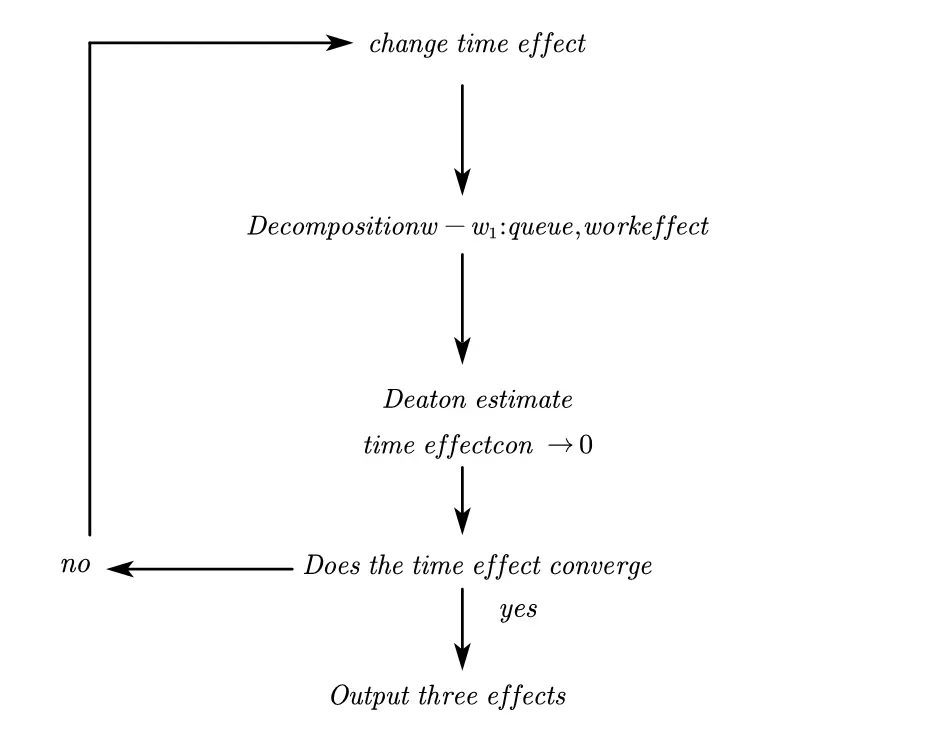
If we look at people’s wage growth from a life cycle perspective, we can put forward a hypothesis: **When a person is about to retire, he will give up any human capital investment. At this time, the source of his wage growth is only the time effect. **At this time, in the two cohorts, within the same $t$ year period, the wage growth rate of the elderly group is 1%; the growth rate of the youth group is 5%, which means that 1% is contributed by the time effect, and 4% is Queue effect + work experience. Then we can study whether the time effect of each group tends to be consistent in old age by continuously adjusting the income effect.

At this time, the depreciation rate $\delta$ can be used for sensitivity testing.