Grouping and Measurement of Econometric Data (STATA Version)

Often, we emphasize the large volume of data, believing that more data means better representation, while neglecting the analysis of data structure, leading to incorrect estimates. Inappropriate estimation methods can result in conclusions that are completely opposite to reality. To better understand data structure, economics has developed fixed effects, moderating effects, heterogeneity analysis, and robustness analysis. These may seem like distinct parts of empirical paradigms, but personally, I believe they all aim to classify data structures to ensure our conclusions are truly valid. Therefore, this article seeks to reorganize the operational significance of empirical papers from the perspective of data structure and variable classification, and to distinguish between different regression commands in STATA.

Below, we introduce an example from Chapter 17, “Measurement,” in Varian’s Microeconomic Analysis.

1. Paradoxes in Statistics

Simpson’s Paradox

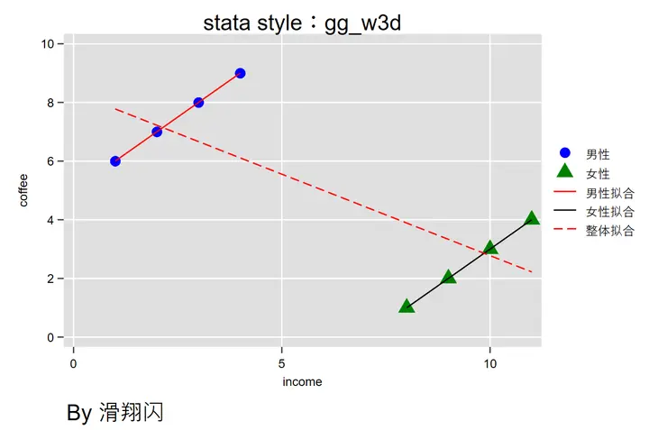
Suppose we want to study the relationship between “coffee consumption and income.” We have data on 4 men and 4 women, along with their income and coffee consumption.

STATA data generation is as follows:

 1
 2
 3
 4
 5
 6
 7
 8
 9
10
11

clear
input str6 gender income coffee
"woman" 8 1
"woman" 9 2
"woman" 10 3
"woman" 11 4
"man" 1 6
"man" 2 7
"man" 3 8
"man" 4 9
end

We can then plot a scatter plot and perform three different sample fits: one for the overall data, one for men, and one for women.

Using this style, STATA can achieve similar effects to R—plotting code is provided below:

1
2
3
4
5
6
7
8
9

*ssc install schemepack, replace  //Painting style command
*For more details, see: https://www.lianxh.cn/news/e76a8a7e3c6c4.html
  set scheme gg_w3d
  
twoway scatter coffee income if gender == "man",color(blue) msize(3) || scatter coffee income if gender == "woman",color(green) msize(3) msymbol(triangle) || lfit coffee income if gender == "man",color(red) || lfit coffee income if gender == "woman" ,color(black) || lfit coffee income ,color(red)  lpattern(dash) ///
		legend(order(1 "Men" 2 "Women" 3 "Men Fit"  4 "Women Fit"  5 "Overall Fit" )) ///
		xtitle("income") ytitle("coffee") ///
		title(stata style：gg_w3d) ///
		note("By 滑翔闪")

If we ignore the details and directly perform regression on the overall data, we might conclude that higher income leads to lower coffee consumption. However, if we perform separate regressions for men and women, the conclusion is the opposite—higher income leads to higher coffee consumption. Clearly, the latter aligns more with reality.

This is $\boxed{Simpson’s Paradox}$: local correlations and overall correlations can present completely different results.

Simpson’s Paradox is ubiquitous in life, such as measuring the efficacy of drugs across different age groups, gender discrimination in college admissions, or racial bias in police enforcement.

• We should not only care about absolute values, such as the gender ratio of a certain outcome;
• But also observe relative values, such as whether police focus more on people of color because they have higher crime rates;

《An alternative test of racial prejudice in motor vehicle searches: Theory and evidence》（2006）¹ is based on “crime rates by race and police enforcement focus” to study racial bias in police enforcement in Florida. Since Floyd’s “I can’t breathe” went viral, many books have used this event to introduce counterfactual inference² (e.g., Mostly Harmless Econometrics by Joshua D. Angrist).

• We should also pay attention to internal stratification, such as by race, region, gender… as in the coffee consumption example above.

One reason for Simpson’s Paradox is omitted variables and confounders³—in the case of coffee consumption and income, gender is an important factor we omitted, but by grouping and fitting, we controlled for it.

Other similar paradoxes include survivorship bias and Berkson’s Paradox… both involve unintentional sample selection that affects analysis results.

2. Panel Data

Cross-sectional data: same time/object, different space; time series: same space/object, different time; panel data: different time, different space/object.
Panel data naturally includes two variables worth discussing—space/object and time.

Economics often uses panel data to analyze reality.

$$ Data\begin{cases} One-dimensional\begin{cases}Time series: time\newline Cross-sectional data: space \end{cases}\newline Two-dimensional (panel data): time + space\newline High-dimensional: more dimensions \end{cases}\newline $$ $$ Panel data\begin{cases} Balanced/unbalanced (whether the ratio of time to space is consistent)\newline Long/short (whether the number of spaces is less than the number of times) \end{cases}\newline $$

For panel data, we first need to clarify which dimension corresponds to time and which corresponds to space/object. It’s essentially a grouping process—you can group by industry or assign each individual a unique ID. In STATA terms, this is:

1

xtset id year

3. Residuals: Economic, Mathematical, and Statistical Meanings

The ordinary regression equation OLS is: $$ Y=\alpha X +u $$ This directly fits the overall data. Knowing Simpson’s Paradox, we understand that such regression is an overall fit and may yield completely different results from local fits. The residual $ \color{red}{u} $ omits too much information we haven’t considered, such as gender classification. Therefore, we need to group the data and decompose the gender variable M from the residual $\color{red}{u}$.

$$ Y=\alpha X +\beta M+u $$ Here, we introduce $\boxed{control variables}$. Note! This is my personal perspective on control variables from a grouping viewpoint, emphasizing their role in selection bias. This grouping requires careful consideration of the practical economic significance of control variables in our study. For example, numerous studies show that coffee consumption habits indeed differ by gender. The selection of control variables also serves to reduce confounding factors; additionally, we must consider optimal fitting, unbiased estimation, and other statistical mathematical meanings.

With panel data, our equation becomes two-dimensional, with object/space coding i and time coding t. The ordinary regression equation OLS becomes: $$ Y_{\color{red}{it}}=\alpha X_{_{\color{red}{it}}}+\beta M_{_{\color{red}{it}}}+u_{_{\color{red}{it}}} $$ To further decompose the economic interpretation of residuals across time and space/object dimensions, we continue to decompose: $$ Y_{\color{red}{it}}=\alpha X _{_{\color{red}{it}}}+\beta M_{_{\color{red}{it}}}+\lambda_{\color{red}{i}}+\gamma_{\color{red}{t}}+u^{\prime } $$ Thus, the equation becomes:

$$ Y_{\color{red}{it}}=\alpha X _{_{\color{red}{it}}}+\beta M_{_{\color{red}{it}}}+\lambda_{\color{red}{i}}+\gamma_{\color{red}{t}}+u^{\prime } $$ First, let’s analyze their economic meaning—variables:

$\boxed{\gamma_{\color{red}{t}}}:$ This part of the residual is the decomposition of the time dimension, indicating that this variation is only related to time, representing time effects. For example, seasonal vegetable yields are clearly related to seasons, and technology naturally progresses steadily over the long term. These effects are shared by all individuals, meaning all samples change synchronously over time.

$\boxed{\lambda_{\color{red}{i}}}:$ This part of the residual is the decomposition of the space/object dimension, indicating that this variation is only related to the individual, representing individual effects. For example, Apple took a long time to adopt USB-C, which is part of their corporate culture. Only Apple had this idea, and for a long time, they were the only company in their industry to insist on this.

$\boxed{u_{\color{red}{it}}^{\prime }}:$ The deviation between the actual value and the estimated value, outside our model’s explanation, is the residual. Causes include measurement errors, omitted variables, and models not aligning with reality…

Next, let’s analyze their mathematical meaning—intercepts:

$$ Y_{\color{red}{it}}=\alpha X_{_{\color{red}{it}}}+\beta D_{_{\color{red}{it}}}+(\lambda_{\color{red}{i}}+\gamma_{\color{red}{t}}+u^{\prime }) $$ Clearly, $(\lambda_{\color{red}{i}}+\gamma_{\color{red}{t}}+u^{\prime })$ as a constant is the intercept in the linear equation structure!

Finally, let’s analyze their statistical meaning—residuals:

Whether there are different intercepts is closely related to the distribution of residuals, heteroscedasticity, and correlation. Fixed effects, random effects, and pooled regressions differ in how they decompose residuals, determining whether our model can explain individual and time effects.

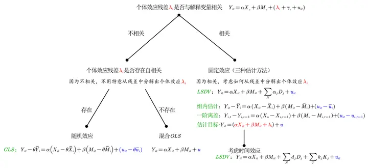
$$ Y_{\color{red}{it}}=\alpha X _{_{\color{red}{it}}}+\beta M_{_{\color{red}{it}}}+(\lambda_{\color{red}{i}}+\gamma_{\color{red}{t}}+u^{\prime }) \newline \xrightarrow{Decomposition} Explainable part + \color{blue}{Unexplainable part} (error) $$ First, here’s a summary chart, followed by an explanation.

Random effects have stricter assumptions, meaning higher data requirements, which is why people tend to use fixed effects (allowing for endogeneity in individual effects).

Through a brief introduction to economic, mathematical, and statistical meanings, we have different decomposition methods for panel data:

$$ Y_{\color{red}{it}}=\alpha X _{_{\color{red}{it}}}+\beta M_{_{\color{red}{it}}}+(\lambda_{\color{red}{i}}+\gamma_{\color{red}{t}}+u^{\prime }) $$

1. Pooled OLS

$\boxed{Pooled OLS}$ : When $Y_{\color{red}{it}}=\alpha X _{_{\color{red}{it}}}+\beta M_{_{\color{red}{it}}}+(\lambda_{\color{red}{i}}+\gamma_{\color{red}{t}}+u^{\prime })=\alpha X _{_{\color{red}{it}}}+\beta M_{_{\color{red}{it}}}+u$, even though we have many methods, such as grouping by year or by individual, we still treat each as a unique data point and pool them together for regression. This can be seen as all data points sharing a single intercept.

Here, we assume no individual effects: $\lambda_{\color{red}{i}}=0$.

We also assume that the remaining residuals are uncorrelated with explanatory and control variables: $Cov（u|M_{_{\color{red}{it}}},X_{_{\color{red}{it}}}） =0$, and the residuals follow a normal distribution.

$$ Y_{\color{red}{it}}=\alpha X _{_{\color{red}{it}}}+\beta M_{_{\color{red}{it}}}+u $$ Pooled OLS uses the least squares method to perform an overall regression on all points, with all data points sharing a single intercept u⁴. Therefore, pooled OLS is also called “longitudinal cross-sectional regression” or “pooled cross-sectional regression.”

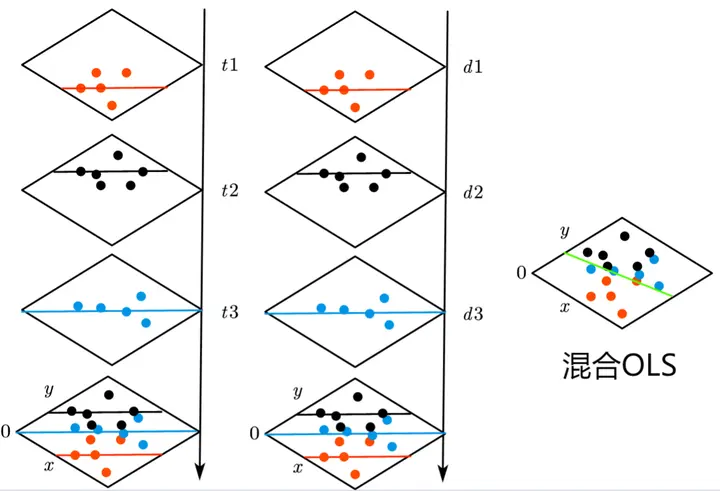
The first column groups by year, with each time section’s data points sharing an intercept; the second column groups by individual, with each individual section’s data points sharing an intercept; the third column’s chart is pooled OLS, where all data points are directly fitted on a single plane.

2. Fixed Effects

Divided into individual fixed effects and time fixed effects (double fixed).

Individual Fixed Effects:

$\boxed{LSDV} :$ Pooled OLS treats all $\lambda_{it}$ equally. Imagine observing the same person multiple times—pooled OLS treats each repeated observation as equally valuable. Fixed effects disagree, believing that individuals have certain traits, and repeated observations provide limited value. Therefore, we need to generate dummy individual variables (n-1) to identify each individual and estimate each individual’s effect separately, known as the “Least Square Dummy Variable Model” (LSDV).

This generates many control variables, so $R^2$ is high.

$$ \begin{align} Y_{\color{red}{it}}&=\alpha X_{\color{red}{it}}+\beta M_{_{\color{red}{it}}}+\alpha_{1}D_{1}+\alpha_{2}D_{2}+\cdots+\alpha_{N}D_{N}+u_{\color{red}{it}}\newline \end{align} $$

Individual effects—causal relationship diagram. Treating individual effects as confounders, we control for them to truncate.

$\boxed{Within-group estimation}$, fixed effects assume that individual effects are correlated with explanatory variables, so we use within-group deviation to eliminate this correlation, similar to de-meaning—subtracting the within-group mean⁵.

The average is taken for the same variable, averaging values across different years: $\bar X_i = \frac{\sum_{t=n}^{t=1}{X_{it}}}{t}$

*Supplement: Frisch-Waugh-Lovell Theorem

The lemma proving that dummy variable least squares and within-group estimation have the same coefficient $\alpha$ is the “Frisch-Waugh-Lovell Theorem.”
Here’s a minimal example:
The real equation is: $$ Y=\beta_1 X_1+ \beta_2 X_2 +u_1 $$ We want to estimate $\beta_1$, but we omitted variable $X_1$ and only regressed $X_2$, resulting in: $$ Y=\alpha X_2+u_2 $$ Now, we regress $X_2$ and $X_1$ to get: $$ X_1=\gamma X_2+u_3 $$ Finally, we regress the residuals: $$ u_2=\dot \beta u_3+u $$ Based on the residuals from the two regressions, we get: $$ \begin{cases} u_2=Y-\alpha X_2\newline u_3 = X_1 - \gamma X_2 \end{cases} $$ Expanding and transforming, we directly obtain: $$ Y=\dot \beta X_1 + (\alpha-\gamma)X_2+u $$ We find that $\dot \beta=\beta_1$, and through this indirect estimation, we estimate the desired coefficient $\beta_1$. Dummy regression first regresses $Y$ with dummy variables $D$, then regresses $X_1$ with $D$, and finally uses residuals for estimation, so the coefficients are consistent with within-group estimation.

FWL proves that first-difference estimation and dummy variable estimation are equal.

If you want to try it yourself, you can use STATA’s built-in data for testing[^6]:

1
2
3
4
5
6
7
8
9

*Use STATA's built-in xtpcse command example data
webuse grunfeld,clear
*If there's no network import, it might be a network issue; you need a VPN.
*Database site: *https://www.stata-press.com/data/r10/xt.html
*You can also download it directly.
reg mvalue invest kstock  i.company
xtreg mvalue invest kstock ,fe
areg mvalue invest kstock , absorb(company)
reghdfe   mvalue invest kstock  , absorb(company)

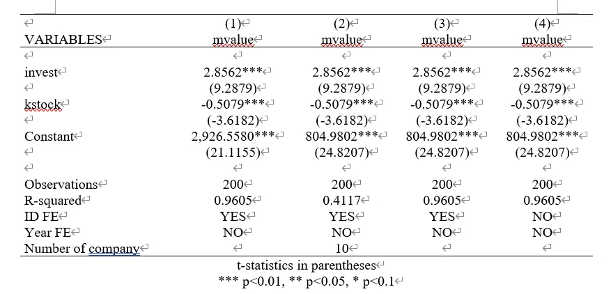
The code blocks use four commands to perform fixed effects, fixing individual effects but not time effects. The results are shown below, and you can see that their coefficient estimates are identical.

Why are the intercepts (constant terms) different?—No explanation was found in any practical books. Personally, I believe[^7] it’s due to different residual calculation methods across commands.

(1) Pooled OLS calculates residuals for one regression equation and all points.

(2) (3) (4) Cluster many regression equations with the same coefficients but different intercepts, and each point calculates variance with its corresponding regression equation, then sums them up.
Why are $R^2$ different:

(1) (3) (4) All use LSDV, so many dummy variables are generated.

(2) Uses between-group estimation, so no dummy variables are generated.

By the way, when we change the code to the following, the situation also changes:

1
2
3
4
5

reg mvalue invest kstock  i.company 
xtreg mvalue invest kstock ,fe r 
areg mvalue invest kstock , absorb(company)  vce(cluster company)
reghdfe   mvalue invest kstock  , absorb(company) 
xtreg laborinput did i.year, fe robust

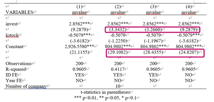
From the image, we can see that the coefficient estimates are the same, but the standard deviations are different.

Default regression uses ordinary standard deviation, requiring data to satisfy homoscedasticity;

Adding r, i.e., robust, uses robust standard deviation to address heteroscedasticity;

Adding vce (cluster company) uses clustered robust standard deviation to address heteroscedasticity + internal autocorrelation.

4. Mechanism Testing

1. The Gray Area of Mechanism Testing in Empirical Studies

Simpson’s Paradox teaches us that grouped regression and overall regression can yield completely different results, partly due to omitted variables. Therefore, we need to add control variables. When using “panel data,” the data includes “time” and “space” dimensions, which can still affect our research. Thus, we need to separate “individual effects” and “time effects.” Answering Simpson’s Paradox—here, we address causality, requiring avoidance of endogeneity. In mechanism testing, some use grouped regression or interaction terms to extend conclusions, assuming—the new variable in mechanism testing is not an omitted control variable.

There’s a big problem here—how do you ensure there’s no endogeneity in mechanism testing? For example, in the figure below, the leftmost path is a collision path in causality, while the right side shows moderating and mediating effects in mechanism testing. Clearly, collision effects with confounders can still satisfy moderating and mediating effects. This introduces a new endogeneity issue!!!! Therefore, Zhu Jiaxiang and Zhang Wenrui (2021)[^8] state that moderating effects do not satisfy statistical causality testing. On this basis, Jiang Ting (2022)[^9] even calls for abandoning the three-step mediation method, as it’s meaningless—it neither proves nor disproves endogeneity.

Thus, our mechanism testing is left with only two options:

1. Further prove no endogeneity. This requires another controlled experiment (feels like another mini economic empirical comparison); or discuss the correlation between residuals and the explained variable after grouped regression. Use correlation + theoretical explanation to approach causality.

2. No need to prove, my variable is naturally exogenous. The variable has no endogeneity in practical terms, meaning more theoretical and economic explanations are needed. The most common “filler” in domestic research is the four major regions and the Hu Line, as these classifications are naturally exogenous variables in practical terms.

It seems that mechanism testing is essentially an incomplete mini-empirical study, extending conclusions through incomplete empirical steps. Personally, I feel that no econometrics textbook emphasizes so-called “mechanism analysis,” but it has become a specific requirement domestically. It seems that quantitative economics ultimately relies on a mix of practical theory and quantitative analysis.

2. Mediation Effects: Differences from Psychological Statistics

The views on mediation effects mainly reference The Book of Why by Judea Pearl.

When we ask why, there are two types of logical chains: one is principle, and the other is process.

$$ Eating oranges\rightarrow Vitamin C\rightarrow Resisting scurvy\newline Elderly\rightarrow Falling\rightarrow Hospitalization\ $$ Taking the above two path diagrams as examples, the first one—eating vitamin C to resist scurvy—sounds more like a principle-based answer, while the elderly falling seems more like a process. I’ve seen many forums and social science自媒体 videos claiming that “economics stole mediation effects from psychology”—this is not the case.

Psychology can widely apply mediation effects because its path diagrams are: $external stimuli\rightarrow human reactions, hormonal changes\rightarrow behavioral changes$, which align more with principles. Economics, on the other hand, answers with $variable1\rightarrow variable2\rightarrow variable3$, which is more like a process description, broader, and less aligned with principles, hence the skepticism. Psychology restricts mediation variables to human performance, while economics has no such strict restrictions, making spurious correlations highly likely. For example, in the case of vitamin C and scurvy, people long believed it was “fruit—oranges” that mattered. The Kost Arctic expedition thought the key was fresh fruit, so they prepared no fruit but only fresh meat, and everyone ended up with scurvy.

To address “Simpson’s Paradox,” we still need mediation effects because of the $\boxed{mediation fallacy}$.

Take the Science paper Sex Bias in Graduate Admissions: Data from Berkeley[^10] as an example. We get the following causal path diagram.

Gender affects admission rates through two paths.

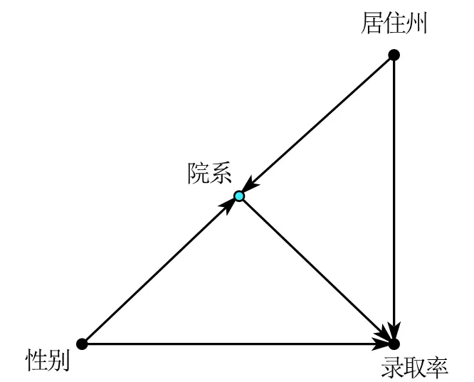
Direct effect: $gender\rightarrow admission rate$

Indirect effect: $gender\rightarrow department\rightarrow admission rate$, where “department” is the mediating variable.

If we directly control for “department,” we show the direct effect of gender on admission rates, and the regression will indicate discrimination against women.

If we only control for “state of residence,” we show the direct effect of gender on admission rates and the indirect effect of gender-department-admission rates, indicating no discrimination against women. The completely different results are precisely Simpson’s Paradox . In the coffee example, we made a mistake by omitting a variable; here, the mistake is controlling for a “mediating variable”. The final conclusion is that because women are more likely to apply to the most competitive departments, their admission rates appear lower, so department is an important mediating variable and should not be casually controlled.

Thus, mediating variables should not be used as control variables, and if we want to distinguish between direct and mediating effects, further differentiation is needed.

3. Moderating Effects: Grouped Regression or Interaction Terms

Found a comprehensive summary

This section mainly references Regression Analysis by Xie Yu.

For variables $Y$, $X_1$, $X_2$, and $D$, we have different estimation strategies.

Grouped regression: $Y=\beta_1 X_1+\beta_2 X_2+u$, then group by D.

Introduce interaction terms, with two estimation methods:

$$ \begin{cases} Y=\beta_1 X_1+\beta_2 X_2+\beta_3D+\beta_4 DX_1+u \newline Y=\beta_1 X_1+\beta_2 X_2+\beta_3DX +u \end{cases} $$

What kind of variables are suitable for interactions?

From a mathematical perspective, addition affects intercepts, while multiplication affects slopes.

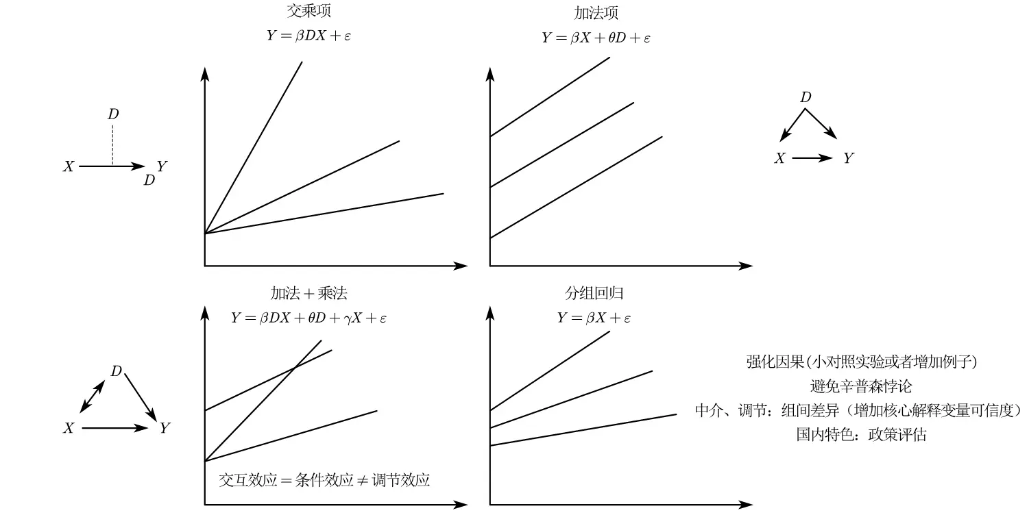
From the figure, moderating effects emphasize interactions because they affect slopes along with X.

Grouped regression emphasizes that X’s slope is the same, only intercepts differ, with no moderating effects, making it more suitable as a control variable.

The above references are from[^2 d]

References:

Introductory Econometrics (Wooldridge)

Basic Econometrics (Gujarati)

Mostly Harmless Econometrics (Angrist / Pischke)

Practical Econometric Methods for Causal Inference (Qiu Jiaping)

Advanced Econometrics and STATA Applications (Chen Qiang)

Regression Analysis (Xie Yu)

The Book of Why (Judea Pearl)

What on Earth Are Interaction Terms in Econometric Regression? Here’s a Book for You

5 Questions and Responses on “Interaction Terms” in Econometrics

STATA: How to Analyze Interaction Terms!

STATA: How to Use Interaction Terms?

STATA: Marginal Effect Analysis

STATA: Visualizing Marginal Effects of Continuous Variables (Interaction Terms)

STATA: Visualizing Interaction/Moderation Effects

After Adding Interaction Terms, the Sign Changed!?