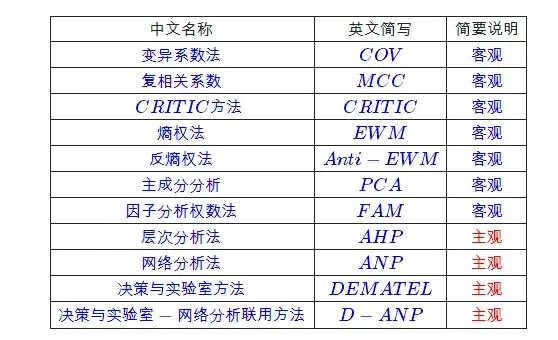
Economic weighting and scoring methods: PCA, CRITIC, EWM

Hupu is popular for “I post pictures, you rate them.” Economics often uses weighting to establish indicators for scoring and comparison. Currently, online tutorials seem to lack one of the three parts: “code-data-derivation”. Here, we aim to cover all three parts at once.

This article first discusses the three most common methods in Chinese journals: “Entropy Weight Method”, “Coefficient of Variation Method”, and “Principal Component Method”. Other methods will be added to this article in the future.

1. “Standardization” and “Normalization”

This section mainly refers to the following blog:

Why are most coupling coordination degree papers wrong?

$\boxed{ Dimensionless }$: No matter how many strange indicators we have initially, we need to present a total score without “units” in the end. This process is called dimensionless.

$\boxed{ Normalization }$: Both “standardization” and “normalization” are used to normalize data, scaling the data into the desired form while preserving the comparative ranking characteristics of the data as much as possible. $$ \small A>B>C>0\xrightarrow{Normalization}\frac{A}{A+B+C}>\frac{B}{A+B+C}>\frac{C}{A+B+C} $$ “Normalization” deals with the range of values, while “standardization” deals with the distribution of values. The comparative ranking characteristics are not changed because they are both linear transformations.

1. Normalization

Transforming data to a specific range to eliminate the impact of different units and numerical gaps on weight analysis.

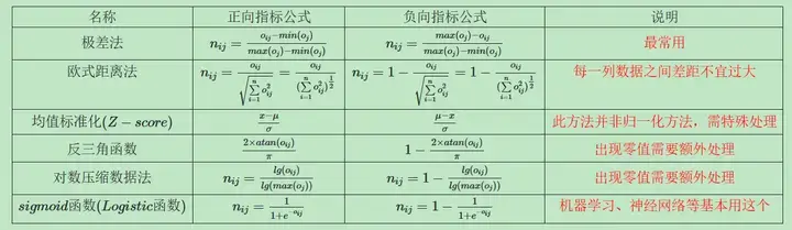
The commonly used formula in economics is as follows: $$ \small \begin{cases} X_{positive\ indicator}=\frac{X_{ij}-\min X_j }{\max X_j-\min X_j}\newline X_{negative\ indicator}=\frac{\max X_j-X_{ij}}{\max X_j-\min X_j} \end{cases}\in{0,1} $$ The range is limited to (0,1). Similarly, to limit the range to a specific interval—(a, b), the transformation is:

$$ \small f(x)\in{0,1} \xrightarrow {Transformation} (b-a)f(x)+a \in {a,b} $$

• Tip 1: Positive and negative indicators require different formulas and should be handled separately.
• Tip 2: There are other normalization methods.

1-1. Normalization Stata Code

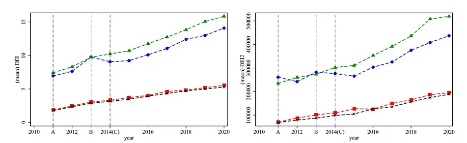
Here, we provide practice data. The data source is Zhao Tao et al. (2020) on digital economy indicators[^1].

Baidu Netdisk

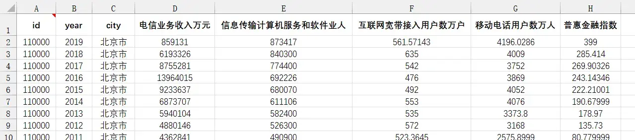
Panel data, five indicators measuring the digital economy

There are many ways to achieve range normalization.

Method 1: Norm Command Group

1
2
3
4

ssc install norm // Command installation
norm x1 x2 x3 , method(mmx) 
* The corresponding calculation method is: [Xi - X(min)]/ [X(max)-X(min)]
* If you want to standardize by group for each cross-section, the command is norm x1 x2 x3, by(year) method(mmx)

The disadvantage of this command is that mmx only provides linear transformation for positive indicators and cannot be used for negative indicators.

That is, only $\small X_{positive\ indicator}=\frac{X_{ij}-\min X_j }{\max X_j-\min X_j}$ is available, and there is no transformation for negative indicators $\small X_{negative\ indicator}=\frac{\max X_j-X_{ij}}{\max X_j-\min X_j} $.

Theoretically, there is a solution: Transform negative indicators into positive indicators through $1-x_{negative\ indicator}$ or $\frac{1}{x_{negative\ indicator}}$ and then perform the transformation uniformly.

Reminder: All data should be positive for scoring.

Method 2: Loop and Group (General)

 1
 2
 3
 4
 5
 6
 7
 8
 9
10
11
12
13
14
15
16
17
18
19
20
21
22
23
24
25
26
27

* Define positive and negative indicators

global positive_var x1  x3 x4 x5 x6  x8 x9 x10 

// Define positive indicators, pack x1 x3 x5 x7 into positive_var

global negative_var x2 x7  

// Define negative indicators, pack x2 x4 x6 x8 into negative_var

global xlist x1 x2 x3 x4 x5 x6 x7 x8 x9 x10 

// Pack all the above indicators into xlist

* Normalization

foreach i in $positive_var {
    qui sum `i'
    gen x_`i'=(`i'-r(min))/(r(max)-r(min)) // Positive indicator normalization
    replace x_`i'=0.000001    if x_`i'==0  // Avoid zero values
  }  

foreach i in $negative_var {
    qui sum `i'
    gen x_`i'=(r(max)-`i')/(r(max)-r(min)) // Negative indicator normalization
    replace x_`i'=0.000001 if x_`i'==0    // Avoid zero values
  }

2. Standardization

$\boxed{Z-score}:$ The central limit theorem tells us that the distribution function tends to be normal. We commonly use standard normalization in probability statistics.

$$ \begin{cases} X_{positive\ indicator}=\frac{x-\mu}\sigma \newline X_{negative\ indicator}=\frac{\mu-x}\sigma \end{cases} $$

2-1. Standardization Stata Code

1
2
3

zscore x1
* The standardized variable is named z_x1
* Negative indicators need to be transformed and then prefixed with a negative sign

When to use standardization and normalization?

TLDR: For machine learning, it depends on the specific object and requirements. For economics, using them without much thought is generally fine.

2. Entropy Weight Method (EWM)

1. Theoretical Steps

First, ensure that the data is normalized and greater than 0. $$ \small \begin{cases} X_{positive\ indicator}=\frac{X_{ij}-\min X_j }{\max X_j-\min X_j} \newline X_{negative\ indicator}=\frac{\max X_j-X_{ij}}{\max X_j-\min X_j} \end{cases}\in{0,1} $$ Then, determine the weights based on the definition of information entropy (from the paper “A mathematical theory of communication”)[^2].

Entropy is actually the mathematical expectation of the bit quantity of a random variable multiplied by the sequential probability of occurrence[^3].

The calculation of information entropy is: $$ \mathrm{E_{j}=-\frac{1}{\ln n}\sum_{i=1}^{n}p_{ij}\ln p_{ij}} $$ $p_{ij} $ is the proportion of each sample in the overall indicator.

$$ p_{ij}=\frac{X_{ij}}{\sum_{i=1}^{n}X_{i}} $$ When $p_{ij}=0$, this formula is not applicable. You can directly supplement the normalized value with a small number to avoid zero values.

Finally, the indicator weight is obtained: $$ W_{i}=\frac{1-E_{i}}{k-\sum E_{i}}(i=1,2,\ldots,k) $$

2. Entropy Weight Method Stata Code

 1
 2
 3
 4
 5
 6
 7
 8
 9
10
11
12
13
14
15
16
17
18
19
20
21
22
23
24
25
26
27
28
29
30
31
32
33
34
35
36
37
38
39
40
41
42
43
44
45
46
47
48
49
50
51
52
53
54
55
56
57
58
59
60
61
62
63
64
65
66
67
68
69
70

*Step0: Define positive and negative indicators

* Define positive and negative indicators

global positive_var x1 x3 x5 x7

// Define positive indicators, pack x1 x3 x5 x7 into positive_var

global negative_var x2 x4 x6 x8

// Define negative indicators, pack x2 x4 x6 x8 into negative_var

global xlist x1 x2 x3 x4 x5 x6 x7 x8 x9 x10 

// Pack all the above indicators into xlist

* Normalization

foreach i in $positive_var {
    qui sum `i'
    gen x_`i'=(`i'-r(min))/(r(max)-r(min)) // Positive indicator normalization
    replace x_`i'=0.000001    if x_`i'==0  // Avoid zero values
  }  

foreach i in $negative_var {
    qui sum `i'
    gen x_`i'=(r(max)-`i')/(r(max)-r(min)) // Negative indicator normalization
    replace x_`i'=0.000001 if x_`i'==0    // Avoid zero values
  }
 
 ************************************Entropy Weight Method*****************************************//
*Step2: Calculate the proportion Pij of the i-th sample value in the j-th indicator to the sum of all sample values of the indicator
foreach i in $xlist {
    egen `i'_sum=sum(x_`i')  // Sum each indicator
    gen y_`i'=x_`i'/`i'_sum  
  }

  gen k=_N  // This code can be modified according to the data type

foreach i in $xlist {
    gen y_lny_`i'=y_`i'*ln(y_`i')  // Indicator proportion multiplied by ln(indicator proportion)
  }

*Step3: Calculate the information entropy ej of the j-th indicator
foreach i in $xlist {
    egen y_lny_`i'_sum=sum(y_lny_`i')  // Sum the indicator proportion multiplied by ln(indicator proportion)
  }

foreach i in $xlist {
    gen e_`i'= -1/ln(k)*y_lny_`i'_sum
  }

*Step4: Calculate the redundancy degree dj of information entropy
foreach i in $xlist {
    gen d_`i'= 1-e_`i'  
  }

*Step5: Calculate the weight wj of the evaluation indicator
egen d_sum = rowtotal(d_*)
foreach i in $xlist {
    gen w_`i'= d_`i'/d_sum
  }

*Step6: Calculate the comprehensive score s
foreach i in $xlist {
    gen Score_`i'= w_`i'*x_`i'   // Weight multiplied by normalized value
  }

egen Score=rowtotal(Score_*)   // Sum
******************************************************************

3. Coefficient of Variation Method (COV)

1. Theoretical Steps

Save time and effort. The coefficient of variation $\boxed{Coefficient\ of\ Variation} $ is the ratio of the standard deviation to the mean for each group.

Calculate the coefficient of variation for each indicator, and then use the proportion of the coefficient of variation as the weight. $$ v_i=\frac{\delta}{\bar x_{i}}
$$

$$ w_i = \frac{v_i}{\sum _{i}^{n} v_i} $$

2. Coefficient of Variation Method Stata Code

 1
 2
 3
 4
 5
 6
 7
 8
 9
10
11
12
13
14
15
16
17
18
19
20
21
22
23
24
25
26
27
28
29
30
31
32
33
34
35
36
37
38
39
40
41
42
43
44
45
46
47
48
49
50
51
52
53
54
55

*Step0: Define positive and negative indicators

* Define positive and negative indicators

global positive_var x1 x3 x5 x7

// Define positive indicators, pack x1 x3 x5 x7 into positive_var

global negative_var x2 x4 x6 x8

// Define negative indicators, pack x2 x4 x6 x8 into negative_var

global xlist x1 x2 x3 x4 x5 x6 x7 x8 x9 x10 

// Pack all the above indicators into xlist

* Normalization

foreach i in $positive_var {
    qui sum `i'
    gen x_`i'=(`i'-r(min))/(r(max)-r(min)) // Positive indicator normalization
    replace x_`i'=0.000001    if x_`i'==0  // Avoid zero values
  }  

foreach i in $negative_var {
    qui sum `i'
    gen x_`i'=(r(max)-`i')/(r(max)-r(min)) // Negative indicator normalization
    replace x_`i'=0.000001 if x_`i'==0    // Avoid zero values
  }
************************************Coefficient of Variation Method*****************************************
*Step2: Calculate the coefficient of variation
foreach i in $xlist {
egen sd_`i'= sd(x_`i') // Calculate standard deviation
}

foreach i in $xlist {
egen mean_`i'= mean(x_`i') // Calculate mean
}

foreach i in $xlist {
gen v_`i'= sd_`i'/ mean_`i' // Calculate coefficient of variation
}

egen v_sum = rowtotal(v_*) // Sum of coefficients of variation

*Step3: Calculate the weight of each indicator
foreach i in $xlist {
gen w_b_`i'=v_`i'/v_sum  
}

*Step4: Calculate the comprehensive score
foreach i in $xlist {
   gen Score_b_`i'= x_`i'*w_b_`i'
}
egen Score_b=rowtotal(Score_b_*)

Personally, I feel that the differences are not significant.

4. CRITIC Method

To be added.

5. Principal Component Score (PCA)

1. Theoretical Steps

Refer to the following articles, which are very well explained.

Principal Component Analysis (PCA) Explained in Detail

CodingLabs - The Mathematical Principles of PCA

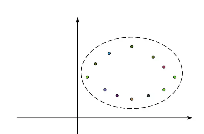
To further visualize the process, we can use two-dimensional data to demonstrate the PCA decomposition process[^4].

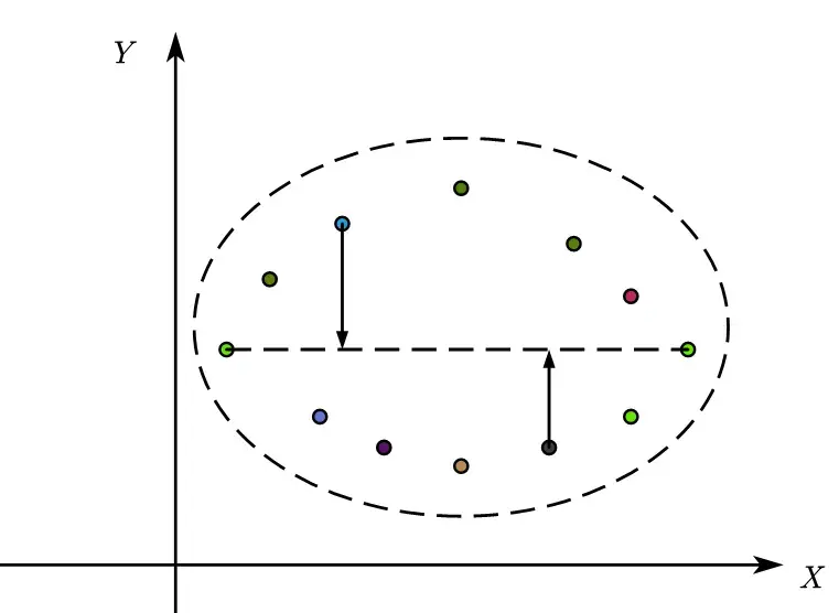
When the data is standardized (standard normal distribution), we obtain a dataset that forms an ellipse.

At this point, we draw a line parallel to the x-axis, making it correspond to the direction with the maximum variance. This principal component $PC_1$ is a linear combination of the two.

$$ PC_1=a_{11}X_1+a_{12}X_2 $$

Similarly, we draw a line parallel to the y-axis, noting that the y-axis is perpendicular to the x-axis to ensure that the two principal components are independent.

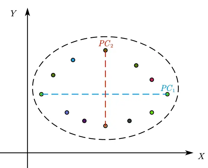
With n indicators, there are n dimensions, and thus n mutually perpendicular directions.

• $\boxed{Eigenvector}:$ The eigenvector is the direction of the axis with the maximum variance (most information), known as the principal component.

• $\boxed{Eigenvalue}:$ The eigenvalue is the variance of a principal component, and its relative proportion can be understood as the explained variance or contribution value. The eigenvalue decreases from the first principal component.

• $\boxed{Loading}:$ The loading is the eigenvector multiplied by the square root of the eigenvalue. The loading is the weight coefficient of each original variable on each principal component.

• $\boxed{Dimension}:$ Dimension in data refers to the number of indicators. With n indicators, there are n dimensions, and thus n mutually perpendicular directions, i.e., n principal components that can be decomposed. However, in practice, we only need a few with significant contributions, so we take k. The process from n to k is $\boxed{Dimensionality\ Reduction} $.

$$ \small \begin{cases} Indicator\ sample\ 1\newline …\newline Indicator\ sample\ n \end{cases} \xrightarrow{Dimensionality\ Reduction} \begin{cases} PC_1=\alpha_1\times f_1+\alpha_2 \times f_2 +…\alpha_3 \times f_n\newline …\newline PC_k=\beta_k \times f_1+\beta_2 \times f_2 +…\beta_n \times f_n \end{cases} $$

2. Principal Component Method Stata Code

Divided into two parts: necessary operations for obtaining scores and non-essential plotting operations.

Important Notes!!!!!!!!!!!!!!!!!!!!

• Stata’s pca command automatically standardizes data, so no additional preprocessing is needed.
• Negative indicators in the analysis data need to be transformed into positive indicators: $\small 1-x_{negative\ indicator} , \small \frac{1}{x_{negative\ indicator}}……$
• The principal component method provides principal components $PC_k$, meaning n indicators are decomposed into k principal components,