Estimating π with a Needle? Notes on Probability Theory (Mao Shisong Edition)

I have been reading Mao Shisong’s “Probability Theory and Mathematical Statistics” these days. Initially, I read the electronic version, but after finishing it, I was so impressed that I immediately bought the physical book. The book truly lives up to its preface in the first edition: the examples are vivid and interesting, and it skillfully explains the tricky variations of each exam point, leaving a deep impression.

Special thanks to the github re-book project team (2019) for the $\LaTeX$ typesetting of the book.

As an introductory book on probability theory and mathematical statistics, we do not want to lead students directly into the mathematical paradise. Instead, we first explore the various landscapes of probability and statistics in the “wild,” and then enter the mathematical paradise, making various concepts and theorems well-grounded and meaningful. This approach allows students to find the book interesting and feel that it is different from reading a typical mathematics textbook. Of course, we also pay great attention to the proofs and discussions of some regularities extracted from randomness, as only by understanding these can one feel them more profoundly.

(First Edition Preface)

Because it is so fascinating, I couldn’t help but record some of the excellent examples from the book on Zhihu.

1. Estimating π with a Needle?

1.1 Introduction: Geometric Probability

For basic notes on classical probability, you can refer to my other answer:

The formula for classical probability is as follows: $$ P(A)=\frac{\text{Number of sample points in event A}}{\text{Total number of sample points in } \Omega}=\frac{k}{n} $$ Geometric probability transforms algebraic formulas into areas (similar to high school linear programming): $$ P=\frac{S_{\text{Area }k}}{S_{\text{Area }n}} $$

Example of Geometric Probability

Divide a line segment of length $a$ into three parts by randomly selecting two points. What is the probability that these three parts can form a triangle?

First, divide the line segment into three parts with lengths $x$, $y$, and $a-x-y$.

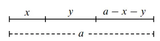
The necessary and sufficient condition for forming a triangle is that the sum of any two sides is greater than the third side, and the difference of any two sides is less than the third side.

Thus, we get the inequality constraints: $$ \begin{cases} 0<a-x-y<x+y\\ 0<x<a-x-y\\ 0<y<x+(a-x-y) \end{cases} \stackrel{\text{Simplified}}{\longrightarrow} \begin{cases} \frac{a}{2}<x+y<a\\ 0<x<\frac{a}{2}\\ 0<y<\frac{a}{2} \end{cases} $$ Now, use $x$ and $y$ to establish a coordinate system and look at the area (similar to linear programming).

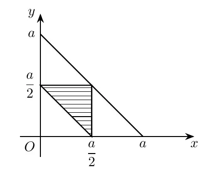
$$ P=\frac{\frac{a^2}{8}}{\frac{a}{2}^2}=\frac{1}{4} $$

1.2 Estimating $\pi$ with a Needle

Buffon’s Needle Problem (famous because the answer is related to $\pi$): On a plane with parallel lines spaced $d(d>0)$ apart, a needle of length $l(l<d)$ is randomly dropped. What is the probability that the needle will intersect one of the parallel lines?

As shown in the figure, the red line represents the needle, and its angle with the horizontal line is $\alpha$.

When the needle intersects a parallel line, take the midpoint of the needle and project it vertically. The projected vertical line segment is divided into two parts.

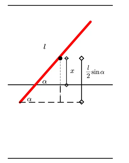
The necessary and sufficient condition for intersection becomes: $x\leq\frac{1}{2}l !sin\alpha$, where the unknown parameters are $x$ and $\alpha$.

The constraints for the parameters are:

$$ \begin{cases} 0 \le x \le d/2\\ 0 \le \alpha \le \pi \end{cases} $$ Establish a coordinate system using these two parameters.

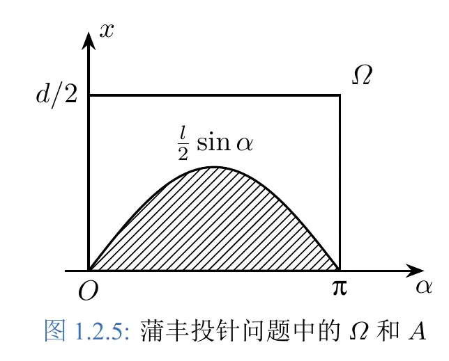
Then, use calculus to find the area of the shaded region and divide it by the area of the rectangle to get the corresponding probability.

$$ P (A) = \frac{S_A}{S_\Omega} = \frac{\int_0^\pi \frac{l}{2} !sin \alpha , \mathrm{d} \alpha}{\frac{d}{2} \pi} = \frac{2l}{d\pi}\\ $$ When $2l=d$, $P (A) =\frac{1}{\pi}$.

Therefore, by conducting more and more experiments and dividing the results, we can estimate $\pi$.

1.3 Supplement: How to Determine Probability

The so-called “Monte Carlo simulation” is a sampling model designed in a computer, where many random values are input and output, and the final frequency is used to approximate the probability.

In Mao Shisong’s textbook, a section is dedicated to discussing methods for determining probability:

• Frequency statistics approximating probability
• Classical methods (permutations, combinations, addition and multiplication principles, etc.)
• Geometric methods
• Subjective methods (e.g., it seems like there’s a 50% chance of rain tomorrow, but the weather forecast says there’s an 85% chance; or saying you have a 60% chance of succeeding at something… these are subjective probabilities)

2. Estimating the Truth in Sensitive Questionnaire Questions

One of the challenges in designing questionnaires is that some questions people are unwilling to answer or provide truthful answers to.

For example, “How often do couples argue?”, “Have you visited inappropriate websites?”, “What is your household income?”… Due to “answers damaging dignity” or “dishonest answers” being beneficial for free-riding (thinking that reporting lower income will result in more government assistance), it is difficult to obtain accurate answers.

Mao Shisong’s probability textbook provides an example when explaining conditional probability, which might make respondents’ answers more effective.

(Although constrained by efficiency, it is probably impractical, but using conditional probability in questionnaire design is an impressive approach.)

2.1 Introduction: Conditional Probability

$$ P(A|B)=\frac{P(AB)}{P(B)}\stackrel{\text{Multiplication Formula}}{\longrightarrow} P(AB) = P(B) P(A|B)\\ $$

$$ \text{Total Probability Formula: } P(A) = \sum_{i=1}^n P(B_i) P(A | B_i)\\ $$

$$ \text{Bayes’ Formula: } P (B_i | A) = \frac{P(B_i) P(A|B_i)}{\sum_{j=1}^n P(B_j) P(A|B_j)} \newline $$

$$ i = 12,\dotsc,n $$

Among the three formulas of conditional probability:

• Multiplication Formula is used to find the probability of the intersection of events.
• Total Probability Formula is used to find the probability of a complex event.
• Bayes’ Formula is used to find a conditional probability.

2.2 How to Operate

The respondent only needs to answer one of the following two questions, with options being “Yes” or “No.”

• Question A: Is your birthday before July 1st?
• Question B: Have you visited inappropriate websites?

(1) The respondent is in a closed room with no other observers, operating and answering questions alone.

(2) The respondent draws a blind box, answering A if a red ball is drawn, and B if a white ball is drawn.

First, we can roughly estimate the probability of “a randomly selected person’s birthday being before July 1st,” which we assume to be 0.5.

Now, with $n$ questionnaires, we have $k$ responses with “Yes,” and the probability of drawing a red ball in the blind box is $\pi$.

That is, we have four data points ($n$, $k$, $\pi$, 0.5).

Now, using the total probability formula:

$$ P(\text{Yes})P(\text{White Ball})P(\text{Yes}|\text{White Ball})+P(\text{Red Ball})P(\text{Yes}|\text{Red Ball}) \stackrel{\text{Substitute Values}}{\longrightarrow} $$

$$ \frac{k}{n}=0.5(1-\pi)+{p_{\text{Yes}|\text{Red Ball}}}\pi \stackrel{\text{Solve}}{\longrightarrow} $$

$$ {p_{\text{Yes}|\text{Red Ball}}}=\frac{\frac{n}{k}-0.5(1-\pi)}{\pi} $$

A cross-disciplinary design of psychology and statistics! A beautiful deception ends here!

3. The Fable of “The Boy Who Cried Wolf” and Bayes’ Formula

3.1 Introduction: Bayes’ Formula

Bayes’ Formula: $$ \text{Bayes’ Formula: } P (B_i | A) = \frac{P(B_i) P(A|B_i)}{\sum_{j=1}^n P(B_j) P(A|B_j)}
$$

$$ i = 1,2,\dotsc,n $$

In Bayes’ formula, if $ P (B_i)$ is called the prior probability of $B_i$, and $P (B_i |A) $ is called the posterior probability of $B_i$, then Bayes’ formula is specifically used to calculate the posterior probability, which is the correction of the probability of $B_i$ based on the new information that $A$ has occurred.

For example, in the story of “The Boy Who Cried Wolf,” the villagers have an initial level of trust in the boy, but after repeated lies, their trust decreases, leading them to not believe the boy even when he tells the truth.

3.2 The Fable of “The Boy Who Cried Wolf”

Let event $A$ be “the boy lies,” and event $B$ be “the boy is trustworthy.”

Assume the villagers’ initial impression of the boy is $P(B)=0.8$, $P(\overline{B})=0.2$.

First, substitute the villagers’ perspective of conditional probability, and assume initial values:

$$ \begin{cases} \text{The boy is trustworthy and lies: } P(A|B)=0.1\\ \text{The boy is untrustworthy and lies: } P(A|\overline{B})=0.5 \end{cases}\ $$ After the boy lies, the villagers will reassess their trust in the boy, so the premise is that the boy has lied, and trust is represented as $P(B|A)$.

After the first lie, substitute into Bayes’ equation:

$$ \begin{align*}
P(B|A) & = \frac{P(B)P(A|B)}{P(B)P(A|B) + P(\bar B)P(A|\bar B) } \\
& = \frac{0.8\times0.1}{0.8\times0.1 + 0.2\times0.5} = 0.444 \end{align*} $$ That is, the villagers’ trust in the boy changes as follows:

$$ \text{Prior Probability} \begin{cases} P(B)=0.8\\ P(\overline{B})=0.2 \end{cases} \stackrel{\text{After one lie}}{\longrightarrow}\text{Posterior Probability} \begin{cases} P(B|A)=0.444\\ P(\overline{B}|A)=0.556 \end{cases} $$ That is, after one lie, the villagers’ trust in the boy becomes $P({B})=0.444$ and $P({B})=0.556$.

Similarly, after the second lie, trust becomes:

$$ P(B|A) = \frac{0.444\times0.1}{0.444\times0.1 + 0.556\times0.5} = 0.138 $$ In summary, after two lies, the villagers’ trust in the boy changes from $P(B)=0.8$ to $P(B)=0.138$.

This is how repeated lies lead to a loss of trust.