
R Basics 1: Interface Introduction and Syntax Structure
 滑翔闪 included in Software Tools and Learning R

R Notes 1: Interface Introduction and Syntax Structure
R Notes 2: Data Cleaning, Plotting, and Econometrics
Notes on my R learning journey. Personally, as an economics learner who only runs regressions, Stata is more than enough1. Whatever it lacks I usually fill with Python wheels, and even for DSGE I use MATLAB’s Dynare add-on. For econometrics, R’s regression table formatting and export are not very friendly, which is a bit of a turn-off.
Although it’s not of much use to me right now, there are three reasons I’m learning it:
- I support open source2, so I wanted to get my feet wet with R;
- I’m currently using RStudio to write my blog files;
- I’ve looked at analyst-type internship postings at big companies like Kuaishou, ByteDance, Tencent, and Baidu, and they generally require using R to handle SQL databases.
Recommended Tutorials
My Recommendations
Forum: Capital of Statistics
Run R code online: Runoob
The foreign counterpart of Runoob: w3schools
A recommended blog site
Strongly recommended: Statistical Software R, an electronic lecture notes by Teacher Li Dongfeng
Strongly recommended: R in Data Science, an electronic lecture notes by Teacher Wang Minjie
Strongly recommended: Introduction to Econometrics with R — the textbook has a strong interactive feel!
Because R can generate websites, many teachers at home and abroad have written their courses as online electronic lecture notes.
Writing a blog is accumulation; writing lecture notes is dedication. There are more and more such teachers, so China should keep getting better too.
See the big collection of R electronic books at bookdown.
Most teachers’ electronic lecture notes will recommend this one.
R project: Mounment’s GitHub repo
Domestic tutorials3, recommended:
I like tutorials that are quick to get into but detailed enough at the key points, and most of the notes in this post come from this video:
After watching the syntax introduction in the video, I suggest going straight to the electronic lecture notes.
The later videos get complicated; no need for them.
Electronic Lecture Notes and Textbooks
Table source: A carefully curated list of the latest and top R books across all fields in 2022
| Field | Top R Books or Resources | Author | Book URL |
|---|---|---|---|
| R Programming | R Programming: Based on the Tidyverse | Zhang Jingxin | https://zhuanlan.zhihu.com/p/467134727 |
| R Programming | R Tutorial | Li Dongfeng | https://www.math.pku.edu.cn/teachers/lidf/docs/Rbook/html/_Rbook/index.html |
| R Programming | Advanced R | Hadley | https://adv-r.hadley.nz/ |
| R Programming | Efficient R programming | Colin Gillespie, Robin Lovelace | https://csgillespie.github.io/efficientR/ |
| R Visualization | ggplot 2: Elegant Graphics for Data Analysis | Hadley | https://ggplot2-book.org/ |
| R Visualization | Interactive web-based data visualization with R, plotly, and shiny | Carson Sievert | https://plotly-r.com/ |
| R Visualization | Modern Statistical Graphics | Zhao Peng, Xie Yihui, Huang Xiangyun | https://bookdown.org/xiangyun/msg/ |
| R Visualization | rstudio:: conf 2020 data visualization workshop | Kieran Healy | https://github.com/rstudio-conf-2020/dataviz |
| R Visualization | R Graphics Cookbook, 2 nd edition | Winston Chang | https://r-graphics.org/ |
| R Visualization | The Beauty of Data Visualization in R | Zhang Jie | https://gitee.com/easyshu/Beautiful-Visualization-with-R |
| Documentation | R Markdown Cookbook | Xie Yihui | https://bookdown.org/yihui/rmarkdown-cookbook/ |
| Documentation | R Markdown: The Definitive Guide | Xie Yihui | https://bookdown.org/yihui/rmarkdown/ |
| Documentation | bookdown: Authoring Books and Technical Documents with R Markdown | Xie Yihui | https://bookdown.org/yihui/bookdown/ |
| R Package Development | R Packages | Hadley | https://r-pkgs.org/ |
| Shiny | Mastering Shiny | Hadley | https://mastering-shiny.org/ |
| Shiny | Engineering Production-Grade Shiny Apps | Colin Fay, Sébastien Rochette, Vincent Guyader and Cervan Girard | https://engineering-shiny.org/ |
| Shiny | JavaScript for R | John Coene | https://javascript-for-r.com/ |
| Applied Statistics | Statistical Inference via Data Science | Chester Ismay and Albert Y. Kim | https://moderndive.com/ |
| Applied Statistics | Introduction to Modern Statistics | Mine Çetinkaya-Rundel | https://openintro-ims.netlify.app/ |
| Applied Statistics | Modern Applied Statistics and R | Huang Xiangyun | https://bookdown.org/xiangyun/masr/ |
| Applied Statistics | Statistics and R (Courseware) | Zhang Jingxin | tidy-R Language Group 2 (222427909) group files |
| Experimental Design | The Grammar of Experimental Designs | Emi Tanaka | https://emitanaka.org/edibble-book/ |
| Bayesian | Doing Bayesian Data Analysis in brms and the tidyverse | A Solomon Kurz | https://bookdown.org/content/3686/ |
| Bayesian | Introduction to Bayesian Econometrics: A GUIded tour using R | Andrés Ramírez-Hassan | https://bookdown.org/aramir21/IntroductionBayesianEconometricsGuidedTour/ |
| Bayesian | An Introduction to Bayesian Reasoning and Methods | Kevin Ross | https://bookdown.org/kevin_davisross/bayesian-reasoning-and-methods/ |
| Bayesian | Statistical rethinking with brms, ggplot 2, and the tidyverse: Second edition | A Solomon Kurz | https://bookdown.org/content/70a06054-8138-4d90-aaa0-895f57aab1b4/ |
| Data Science | R for Data Science | Hadley | https://r4ds.had.co.nz/ |
| Data Science | Tidyverse Skills for Data Science in R | Carrie Wright, Shannon Ellis, Stephanie Hicks, and Roger D. Peng | https://leanpub.com/tidyverseskillsdatascience |
| Data Science | R in Data Science | Wang Minjie | https://bookdown.org/wangminjie/R4DS/ |
| Data Science | Data Science Live Book | Pablo Casas | https://livebook.datascienceheroes.com/ |
| Data Science | R in Action (Third Edition) | Rob Kabacoff | https://livebook.manning.com/book/r-in-action-third-edition/ |
| Data Science | Modern Data Science with R (2 nd) | Benjamin S. Baumer, Daniel T. Kaplan, and Nicholas J. Horton | https://mdsr-book.github.io/mdsr2e/ |
| Machine Learning | mlr 3 book | Official | https://mlr3book.mlr-org.com/ |
| Machine Learning | Tidy Modeling with R | MAX KUHN AND JULIASILGE | https://www.tmwr.org/index.html |
| Machine Learning | Hands-On Machine Learning with R | Bradley Boehmke & Brandon Greenwell | https://bradleyboehmke.github.io/HOML/ |
| Machine Learning | Feature Engineering and Selection: A Practical Approach for Predictive Models | Max Kuhn and Kjell Johnson | http://www.feat.engineering/ |
| Machine Learning | An Introduction to Statistical Learning with R | Gareth James, Daniela Witten, Trevor Hastie, Robert Tibshirani | https://trevorhastie.github.io/ISLR/ |
| Machine Learning | Machine Learning with R: Based on mlr 3 verse (Courseware) | Zhang Jingxin | tidy-R Language Group 2 (222427909) group files |
| Deep Learning | Deep Learning with R, Second Edition | François Chollet with Tomasz Kalinowski and J. J. Allaire | https://www.manning.com/books/deep-learning-with-r-second-edition |
| Text Mining | Supervised Machine Learning for Text Analysis in R | EMIL HVITFELDT AND JULIA SILGE | https://smltar.com/ |
| Text Mining | QUANTEDA TUTORIALS | Kohei Watanabe and Stefan Müller | https://tutorials.quanteda.io/ |
| Text Mining | Text Analysis Tutorials | LADAL | https://slcladal.github.io/index.html |
| Econometrics | Introduction to Econometrics with R | Christoph Hanck, Martin Arnold, Alexander Gerber, and Martin Schmelzer | https://www.econometrics-with-r.org/ |
| Econometrics | Beyond Multiple Linear Regression: Applied Generalized Linear Models and Multilevel Models in R | Paul Roback and Julie Legler | https://bookdown.org/roback/bookdown-BeyondMLR/ |
| Econometrics | Mixed Models with R Getting started with random effects | Michael Clark | https://m-clark.github.io/mixed-models-with-R/ |
| Time Series | Forecasting: Principles and Practice (3 rd ed) | RobJHyndman | https://otexts.com/fpp3/ |
| Time Series | Lecture Notes on Financial Time Series Analysis | Li Dongfeng | https://www.math.pku.edu.cn/teachers/lidf/course/fts/ftsnotes/html/_ftsnotes/index.html |
| Finance | Tidy Finance with R | Christoph Scheuch, Stefan Voigt, and Patrick Weiss | https://tidy-finance.org/ |
| Spatial Data Analysis | Geocomputation with R | Robin Lovelace, Jakub Nowosad, Jannes Muenchow | https://geocompr.robinlovelace.net |
| Spatial Data Analysis | Spatial Data Science with applications in R | Edzer Pebesma, Roger Bivand | https://keen-swartz-3146c4.netlify.app/ |
| Spatial Data Analysis | NHH ECS 530 2021 course: Spatial data analysis (with R) | Roger Bivand | https://rsbivand.github.io/ECS530_h21/ |
| Causal Inference | The Effect: An Introduction to Research Design and Causality | Nick Huntington-Klein | https://theeffectbook.net/ |
| Causal Inference | Causal Inference: The Mixtape | Scott Cunningham | https://mixtape.scunning.com/index.html |
| Social Sciences | Data Analytics for the Social Sciences Applications in R | G. David Garson | |
| Social Sciences | A Business Analyst’s Introduction to Business Analytics | Adam Fleischhacker | https://www.causact.com/ |
| Social Sciences | Computing for the Social Sciences | Benjamin Soltoff | https://cfss.uchicago.edu/notes/intro-to-course/ |
| Network Analysis | Methods for Network Analysis | Mark Hoffman | https://bookdown.org/markhoff/social_network_analysis/ |
| Network Analysis | Handbook of Graphs and Networks in People Analytics: With Examples in R and Python | Keith McNulty | https://ona-book.org/ |
| Network Modeling | workshop 2020_Network Modeling for Epidemics | http://statnet.org | https://statnet.org/nme/d1.html |
| Model Computation | Model Estimation by Example Demonstrations with R | Michael Clark | https://m-clark.github.io/models-by-example/ |
| Model Computation | Computer-age Calculus with R | Daniel Kaplan | https://dtkaplan.github.io/RforCalculus/ |
| Big Data | Mastering Spark with R | Javier Luraschi, Kevin Kuo, Edgar Ruiz | https://therinspark.com/ |
| Meta-Analysis | Doing Meta-Analysis in R: A Hands-on Guide | Harrer, M., Cuijpers, P., Furukawa, T.A., & Ebert, D.D | https://bookdown.org/mathiasHarrer/Doing_Meta_Analysis_in_R/ |
| Survival Analysis | Applied Survival Analysis Using R | Dirk F. Moore |
Downloading R
My environment:
R (the language itself) + RStudio (IDE) + Rtools (package management, Windows only)
Downloading is simple — just click through and say yes all the way.
R itself: https://cran.r-project.org/
RStudio desktop software: https://posit.co/download/rstudio-desktop/
R itself comes with Chinese support, but RStudio doesn’t. There’s a Chinese localization GitHub project, but it doesn’t work well and I don’t recommend it — you’ll get crashes and incompatibility bugs, which is a hassle.
RStudio Interface and Setup
Interface Introduction
Menu path for page settings: tools - global option - Pane Layout
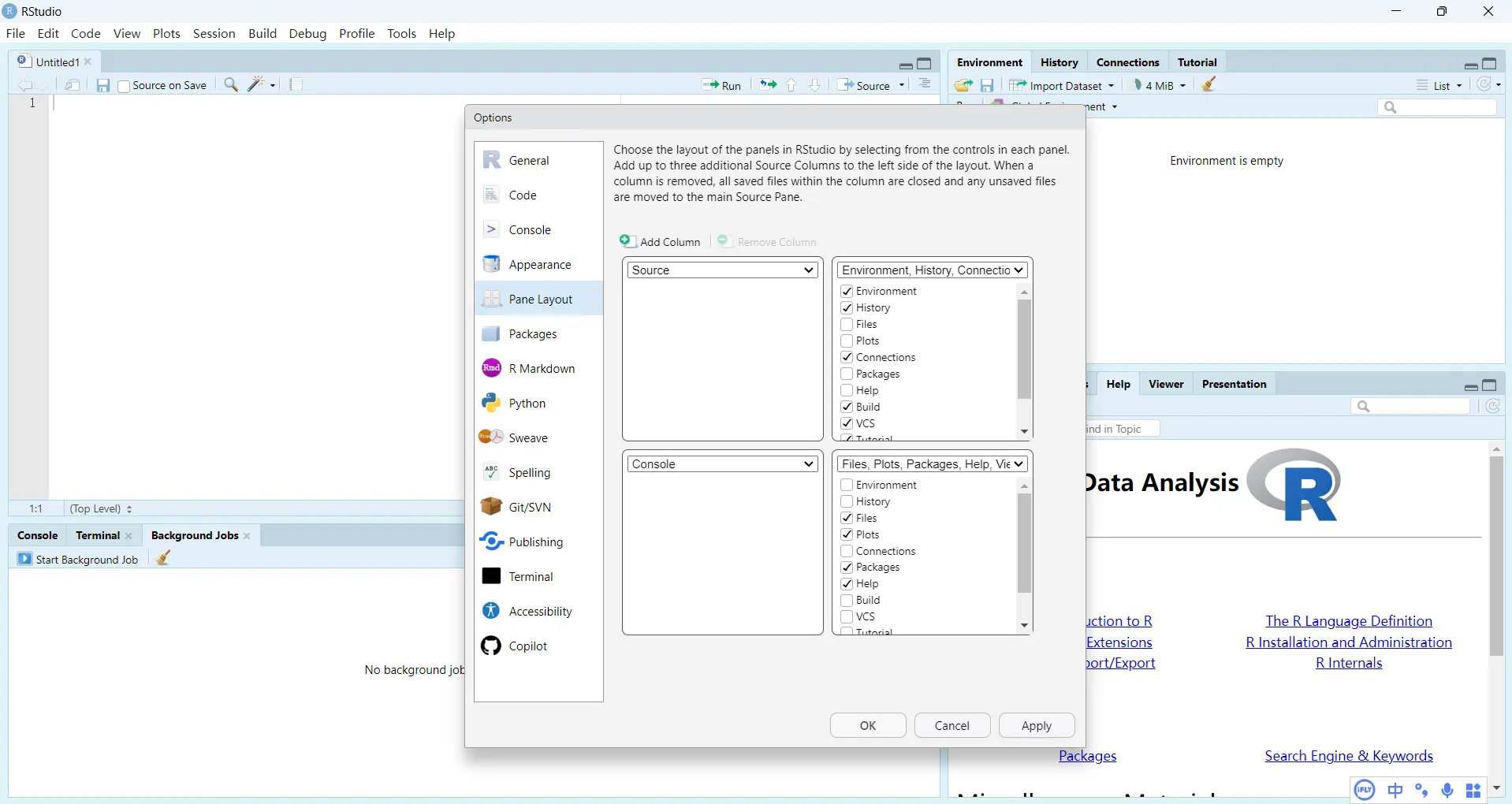
At this point,
The source panel in the top-left (after creating a new R script project) is where you write code.
The console in the bottom-left shows the results.
The top and bottom sections on the right are customizable panels. For example, history shows your code run history; environment is the variable environment, where you can use import Dataset to load Stata, Excel, and other data; file shows the computer directories of your working environment.
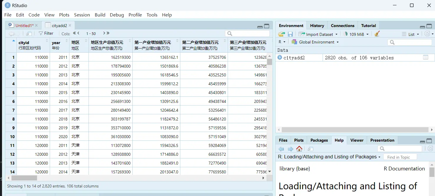
Managing and Downloading Packages
Manual Installation
Using R over the long term is tough on your computer’s storage, because you keep downloading packages.
On Windows, R is generally managed with Rtools. Recent versions of R should come with this toolkit; if not, just install it from the official site — just install the .exe.
In the file panel, there’s a Packages section; click install there to install packages.
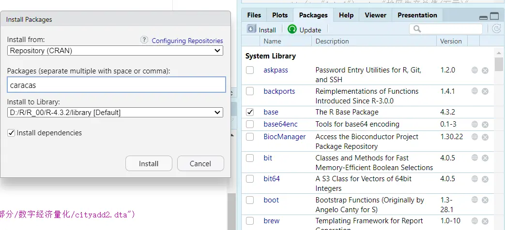
Installing and Loading via Commands
R is a language for statisticians. I personally find its base syntax not very elegant, but since it’s open source, once you load the right packages it becomes a real joy.
For example, to install the car package, you can use the following commands:
| |
Since different packages may have functions with the same name, when loading two packages causes a conflict, the same-named function from the later package will override the earlier one.
Setting the Working Directory
| |
Loading Data
In Stata, one window can only load one dataset, but R can load multiple.
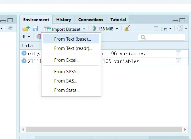
| |
Syntax
Data Types
| Type | Example or Description | Type |
|---|---|---|
| Numeric | 2333 233.3 | numeric |
| Character | ‘Next one is you’ “JOJO” “2333” | character |
| Logical | TRUE T FALSE F | logical |
| Missing value | For example, forcing text into a number fails | NA |
| Blank value | NULL | |
| Not a number | Not a Number | NaN |
| Infinity | abbreviation of “Infinite” | Inf |
| |
Data Structures
Assignment and Vectors
The usual order of introduction: assignment, indexing, slicing.
| |
Matrices
Matrices are just vector commands stacked together.
| |
Lists
Unlike vectors and matrices, lists can combine different data types and structures.
| |
Data Frames
A special kind of list — the panel data and time series we often work with are built using data frames.
| |
Basic Operations and Functions
Basic Operations
| |
Vector Function Operations
| |
Data Frame and Matrix Operations
Data Frame
| |
Matrix
| |
Character Functions
| |
Distribution Functions
| |
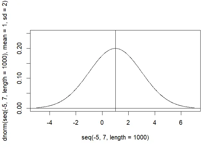
Basic Syntax
Loops
Stata simplifies this to local, global, and foreach for looping over variables; the downside is that it’s not convenient for adding and subtracting across rows.
| |
Conditionals
If-else is old hat, so I won’t give too many examples here.
| |
Writing Functions
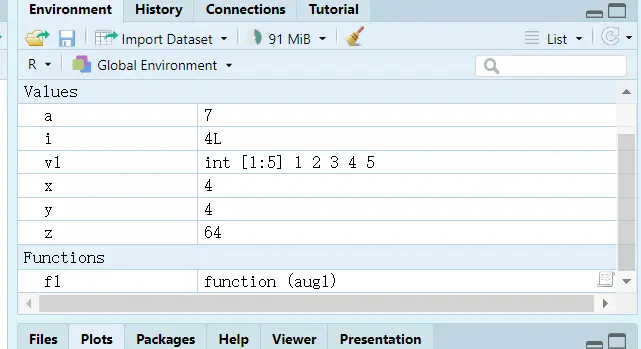
| |
Data Wrangling
The tidyverse package’s official site: https://www.tidyverse.org/
You can download the test dataset here: https://moxingjiqi.shinyapps.io/dataset/
The haven package in tidyverse supports reading SPSS, Stata, and SAS.
It’s best not to include Chinese characters in file paths, otherwise you can easily get garbled text and import failures.
Import and Export
Table source: R in Data Science
| Format | Command |
|---|---|
| .txt | read.table() |
| .csv | read.csv() and readr::read_csv() |
| .xls and .xlsx | readxl::read_excel() and openxlsx::read.xlsx() |
| .sav (SPSS files) | haven::read_sav() and foreign::read.spss() |
| .Rdata or rda | load() |
| .rds | readRDS() and readr::read_rds() |
| .dta | haven::read_dta() and haven::read_stata() |
| .sas 7 bdat (SAS files) | haven::read_sas() |
| Internet | download.file() |
| |
At least the vast majority of journal master files are do-files. As for plotting, Stata’s
schemepackpackage is already powerful enough to be adjusted to R’s default style. ↩︎Using Zotero for reference management was the start of my love for the open-source philosophy. ↩︎
Selling courses in China really is second to none. ↩︎