Common databases and cleaning ideas were already introduced in the Stata version; here I focus on recording commonly used R code for data cleaning.
While organizing this, I kept feeling the power of open source. Every task has a native R trick, but all sorts of packages keep popping up to save you effort, so…
Even if guidance has shattered, please become the king of package-calling!
Data Cleaning
Working Directory
1
2
3
4
5
6
7
8
# Clear all variablesrm(list=ls())# View the current directorygetwd()# Set the working directory; note that forward slashes are usedsetwd("F:/桌面")# Get a file path; this opens a file browser to find the file manually, and clicking it returns the file pathfile.choose()
### 1. read.rable() #### Read from txt, with "\t" as the delimiter# head means viewing the first few rowstes=read.table("./data/top250.txt",header=TRUE,sep="\t",fileEncoding="GBK");head(tes)### 2. read.csv() #### Dedicated function read.csvmovie_csv=read.csv("./data/top250.csv",fileEncoding="GBK");head(movie_csv)library("readxl")# Load the package# The col_names parameter is again used to set whether the first row is treated as variable namesmovie_excel=data.frame(read_excel("./data/top250.xlsx",col_names=TRUE));head(movie_excel)
# Get csv files in bulklibrary(readr)library(dplyr)# Set the folder pathfolder_path<-"F:/桌面/文件夹/"# Get the paths of all csv files in the foldercsv_files<-list.files(folder_path,pattern="\\.csv$",full.names=TRUE)# Create an empty list to store the read csv datadata_list<-list()# Loop through and read each csv file, storing it in data_listfor(fileincsv_files){data<-read_csv(file)data_list[[file]]<-data}# Combine all the data into one data framecombined_data<-bind_rows(data_list)# View the combined dataprint(combined_data)#————————————————————————————————————————————————————# Get xlsx files in bulklibrary(readxl)library(dplyr)# Set the folder pathfolder_path<-"F:/桌面/文件夹/"# Get the paths of all xlsx files in the folderxlsx_files<-list.files(folder_path,pattern="\\.xlsx$",full.names=TRUE)# Create an empty list to store the read xlsx datadata_list<-list()# Loop through and read each xlsx file, storing it in data_listfor(fileinxlsx_files){data<-read_excel(file)data_list[[file]]<-data}# Combine all the data into one data framecombined_data<-bind_rows(data_list)
Checking Data Types
1
2
3
4
5
names(中国城市数据库)# View the column numbers corresponding to the variable namesstr(中国城市数据库)# Check the data typessummary(中国城市数据库)# Max, min, and mean; only supports numeric columnssummary(中国城市数据库[,c(2,4:6)])# View column 2 and columns 4 to 6summary(中国城市数据库[,2:12])# View columns 2 to 12
Renaming Variables
The simplest method — select
Note! We want to rename the column 年份 to year, i.e., the assignment is year = 年份!
If the file contains special symbols, wrap them with `` symbols
By the way, here’s a more complicated way to rename (basic R syntax):
1
2
3
4
5
# Rename the first column to bbsetwd("F:/桌面/R")中国城市数据库 <-readxl::read_excel("中国城市数据库.xlsx")colnames(中国城市数据库)[1]<-'bb'# Similarly, row names are changed with rownames
Using dataset$column_name is how you specify a column variable; many of RStudio’s features are quite handy
If a variable name is too long and we don’t know which column the variable to rename is in, use names(中国城市数据库); the result will show the variable names and their corresponding column numbers.
Creating New Variables
I recommend Method 1.
Method 1
1
2
3
d3<-mutate(中国城市数据库,year= 年份/2)
Method 2
1
2
3
4
5
6
7
8
9
# Mainly use transform()# The first argument is the name of the data frame to operate on# The following arguments are the operation formulas# The left side of the formula is the new variable name# The right side of the formula is the specific operationmydata<-transform(mydata,sum=x1+x2,mean=(x1+x2)/2)
Method 3
1
2
3
4
mydata$mean<-(mydata$x1+mydata$x2)/2# Create a new variable named mean, obtained by averaging the two original variables (x1 and x2)mydata$empty_variable<-NULL# Create an empty variable
Extracting and Appending Characters
Create a new variable x by extracting a string of length 4 from variable var starting at position 1.
1
2
3
4
5
6
7
8
中国城市数据库 <- 中国城市数据库 %>%mutate(x=substr(var,1,4))# Append at the end 中国城市数据库2<- 中国城市数据库2%>%mutate(x=paste0(var,"_suffix"))# Add at the front中国城市数据库2<- 中国城市数据库2%>%mutate(x=paste(var,"_suffix"))
Data Type Conversion
Including date conversion.
1
2
3
4
5
mydata$x<-as.factor(mydata$x)# Other typesas.numeric('123')as.character(123)as.logical(FALSE)
Dates and Times
Date Conversion
1
2
3
as.Date('1/15/2020',format='%m/%d/%Y')###(2) Convert characters to POSIXct/POSIXlt time format ###as.POSIXct(1472562988,origin="1960-01-01")# Convert a date value, using "1960-01-01" as the origin
Extracting Date Components
 1
 2
 3
 4
 5
 6
 7
 8
 9
10
11
12
13
14
15
16
17
library(lubridate)# Load the lubridate packaget="2020-11-20 01:30:29"year(t)# Extract the year## [1] 2020month(t)# Extract the month## [1] 11mday(t)# Extract the day of the month## [1] 20wday(t)# Extract the day of the week## [1] 6hour(t)# Extract the hour## [1] 1minute(t)# Extract the minute## [1] 30second(t)# Extract the second## [1] 29
Date Calculations
1
2
3
4
5
6
7
8
9
10
# Find the number of days between any two datesbegin=as.Date("2016-03-04")end=as.Date("2016-05-08")(during=end-begin)## Time difference of 65 days# Find the number of weeks and hours between any two datesdifftime(end,begin,units="weeks")## Time difference of 9.285714 weeksdifftime(end,begin,units="hours")## Time difference of 1560 hours
Sorting, Selecting, and Grouping
Filtering Rows
1
2
3
4
# Select rows in mydata with year 2020 and cityid >= 1100filter(mydata,year==2020,cityid>=1100)# Exclude rows in mydata with year 2020 or cityid >= 1100filter(mydata,!(year==2020|cityid>=1100))
Selecting Columns
1
2
# Drop the columns from year to cityidselect(mydata,-(year:cityid))
Sorting
1
2
3
4
5
# Sort by GDPorder(中国城市数据库$$地区生产总值.万元.)# When a variable name contains (), use .. in place of the name so R can recognize it# Sort by GDP in descending ordersorted_values<-sort(中国城市数据库$地区生产总值.万元.,decreasing=TRUE)
Grouped Processing
1
2
3
4
5
6
7
8
9
10
11
12
library(dplyr)# Use the dplyr package to compute group means中国城市数据库 <- 中国城市数据库 %>%group_by(国界)%>%mutate( 乡村振兴边境 =mean(乡村振兴,na.rm=TRUE), 产业兴旺边境 =mean(产业兴旺,na.rm=TRUE), 生态宜居边境 =mean(生态宜居,na.rm=TRUE), 治理有效边境 =mean(治理有效,na.rm=TRUE), 乡风文明边境 =mean(乡风文明,na.rm=TRUE), 生活富裕边境 =mean(生活富裕,na.rm=TRUE))
Matching and Merging
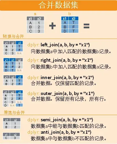
Although R has a built-in merge similar to Stata’s, it’s weaker and can only do one-to-one matching, so I recommend the dplyr package here.
Horizontal
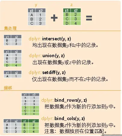
Vertical
1
2
3
4
5
6
7
8
9
10
11
12
13
14
15
16
17
18
19
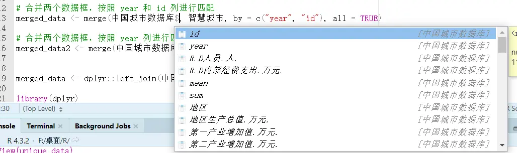
library(dplyr)# Horizontaldplyr::left_join(a,b,by="x1")dplyr::right_join(a,b,by="x1")dplyr::inner_join(a,b,by="x1")dplyr::outer_join(a,b,by="x1")dplyr::semi_join(a,b,by="x1")dplyr::anti_join(a,b,by="x1")# Verticaldplyr::intersect(a,b)dplyr::union(a,b)dplyr::setdiff(a,b)dplyr::bind_rows(a,b)# Example# Match city data and pilot policy by id and year# For partial matching, slice by index [m,n:l]merged_data<-dplyr::left_join(中国城市数据库, 智慧城市,by=c("year","id"))merged_data2<-merge(中国城市数据库[,3:5], 智慧城市,by="year",all=TRUE)
na.rm = TRUE is a parameter usually used to specify whether to remove missing values when performing calculations on data. When the na.rm parameter is set to TRUE, the function removes missing values from the data before computing; when it is set to FALSE or omitted, the function includes the missing values and returns NA as the result.
Cross-Sectional Interpolation
1
2
3
4
5
6
7
8
# Replace missing values in the gdp column of 中国城市数据库 with the column mean中国城市数据库[is.na(中国城市数据库$gdp),]$gdp<-mean(中国城市数据库$gdp,na.rm=TRUE)# Replace outliers less than 0 in the score column of 中国城市数据库 with missing values中国城市数据库[which(中国城市数据库$score<0),]$score<-NA# Replace missing values in the score column of 中国城市数据库 with the column mean中国城市数据库[is.na(中国城市数据库$score),]$score<-mean(中国城市数据库$score,na.rm=TRUE)
Panel Interpolation
Referring to Stata’s interpolation command, I found a similar interpolation method in R.
1
2
3
4
5
6
7
8
9
10
11
12
library(dplyr)library(zoo)# Treat the data frame as panel data, group by id and year, and interpolate "地区生产总值.万元."中国城市数据库_new<- 中国城市数据库 %>%arrange(id,year)%>%group_by(id)# Interpolation中国城市数据库_new<- 中国城市数据库_new%>%mutate(地区生产总值.万元.=na.approx(地区生产总值.万元.))# Extrapolation中国城市数据库_new<- 中国城市数据库_new%>%mutate(地区生产总值.万元.=na.approx(地区生产总值.万元.,method="constant"))
Values beyond a specific range are replaced with the value at the boundary of that range.
1
2
3
4
5
6
7
8
9
10
library(statar)statar::winsorize(v,probs=c(0.01,0.99))# R can also first compute the data distribution and then delete based on it# Compute the percentilesquantiles<-quantile(中国城市数据库2$R.D内部经费支出.万元.,probs=c(0.01,0.99))# Replace the extreme values中国城市数据库2$R.D内部经费支出.万元.[中国城市数据库2$R.D内部经费支出.万元.<quantiles[1]]<-quantiles[1]中国城市数据库2$R.D内部经费支出.万元.[中国城市数据库2$R.D内部经费支出.万元.>quantiles[2]]<-quantiles[2]
Deleting Data
Delete blank values and values that don’t apply to the questionnaire.
Since Stata can only operate on one table at a time, you add and remove everything on a single table; but R supports working with multiple tables, so in practice filtering is achieved by extracting the appropriate data to form a new table.
1
2
3
4
5
6
7
8
9
10
11
# Delete the rows with year 2020, and drop columns 5 and 10中国城市数据库_new<- 中国城市数据库[中国城市数据库$year!="2020",-c(5,10)]# Use a loop function# Create a character vector containing the variable names to be imputedvar<-c("var0","var1","var2","var3","genshin")# Loop through each variable namefor(iinvar){# Delete specific values in the variabledata<-subset(data,!(data[,i]==-88|data[,i]==-99|is.na(data[,i])|data[,i]<=0))}
ggplot2 is about divide-and-conquer plotting, so its syntax consists of
$$
Step 1 (specify the dataset, specify the axes) + Step 2 (specify the plot type) + Plot 3 (decoration) + Combination 4 (......)
$$
The general steps for plotting with ggplot2 are:
Prepare the data, usually a data frame, and generally in long format, i.e., each observation time takes one row and each observed variable takes one column.
Input the data into the ggplot() function, and specify which graphical attributes each variable in the plot maps to, such as the x coordinate, y coordinate, color, shape, etc. These mappings are called aesthetic mappings, or aesthetics.
Choose a suitable plot type; the function name starts with geom_, such as geom_point() for a scatter plot. The plot type is called a geom for short. Connect the ggplot() part and the geom_xxx() part with a plus sign. You can already make a plot at this point; the following steps are further refinements.
Set an appropriate coordinate system, such as coord_cartesian(), scale_x_log10(), etc. Again connect with a plus sign.
Set the title, legend position, and so on, such as labs(). Again connect with a plus sign.
The syntax really doesn’t feel as clean and convenient as Stata’s (
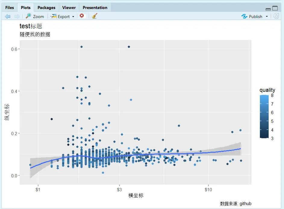
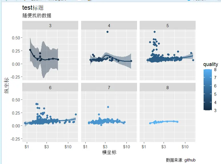
geom_point(): scatter points; similarly, add a line plot with geom_line()
geom_smooth(): fitted line
scale_x_log10: log-transform the x-axis with base 10
color = quality: fill colors by group according to the quality variable
facet_wrap(~ quality): slice into groups by the quality variable; it can also be (a~b), which is two-dimensional grouping. You can also use facet_grid(row variable ~ column variable).
setwd("F:/桌面/R")testdata<-readr::read_csv("wineQualityReds.csv")names(testdata)library(ggplot2)# qplot for quick plottingqplot(x=chlorides,y=chlorides,data=testdata,geom="point")# Plot with ggplotp<-ggplot(data=testdata,mapping=aes(x=residual.sugar,y=chlorides,color=quality,fill=quality))p1<-p+geom_point()+geom_smooth(method="loess")+scale_x_log10(labels=scales::dollar)+labs(x="横坐标",y="纵坐标",title="test标题",subtitle="随便找的数据",caption="数据来源: github")+facet_wrap(~quality)print(p1)ggsave(filename="文件名.png")
Scatter plot with a fitted line
After faceting
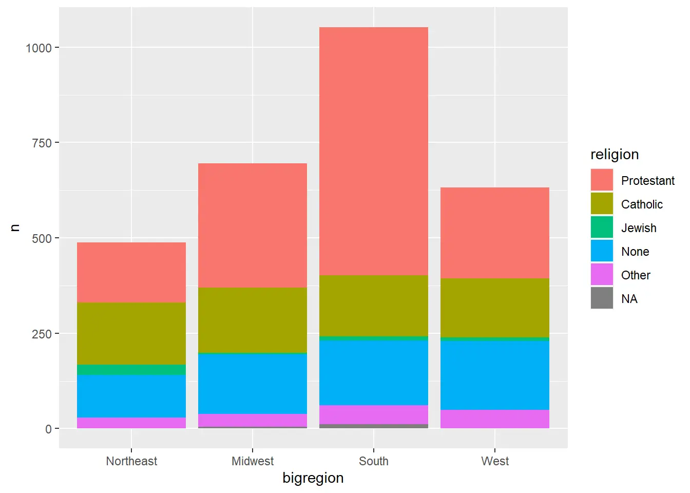
Bar Charts
1
2
3
4
5
6
7
8
9
10
11
12
13
14
15
16
17
18
19
# Count using the dataset数据集 <- 原始数据集 |>select(分类变量)|>count(分类变量)|>mutate(比例值 =n/sum(n))p<-ggplot(数据集,aes(x= 分类变量
y=n,# Can also change to the ratio valuefill=religion# Different categories in different colors ))p+geom_col()+labs(y="纵坐标名字")+guides(fill="none")# Whether to remove the legend+coord_flip()# Swap the x and y axes+geom_col(position="stack")# Stack+facet_grid(A~B)# Facet into groups
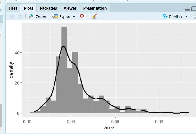
# midwest is a dataset bundled with ggplot# Histogramp<-ggplot(midwest,aes(x=area))p+geom_histogram()# Kernel density plotggplot(midwest,aes(x=area,color=state,fill=state))+geom_density(alpha=0.3)# alpha = 0.3 sets the transparency# Histogram with kernel densityggplot(midwest,aes(x=area))+geom_histogram(mapping=aes(y=..density..),alpha=0.6)+geom_density(size=1.1)
Histogram with a kernel density line added
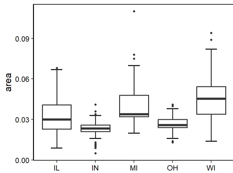
Box Plots
1
2
3
4
5
6
7
8
9
10
# Just change ggplot(dataset, aes(categorical x, target y))p<-ggplot(midwest,aes(state,area))+stat_boxplot(geom='errorbar',width=0.3,cex=1)+#errorbargeom_boxplot(cex=1)+labs(x=NULL)+theme_classic(base_size=18)+theme(panel.border=element_rect(size=1,fill='transparent'),legend.position='none',axis.text=element_text(color='black'))# Theme adjustmentsp
# Load the package library(ggcorrplot)cormtcars<-round(cor(mtcars),3)# round() sets the number of decimal placesggcorrplot(cor(cormtcars))# The default is squares; change to circles and add the correlation coefficientsggcorrplot(cormtcars,method="circle",lab=T)# Use the cor_pmat() function from the ggcorrplot package to compute p-values:pmtcars<-cor_pmat(mtcars)ggcorrplot(cormtcars,hc.order=T,# Hierarchical clustering to reorder the matrixggtheme=ggplot2::theme_void(base_size=15),# Theme changescolors=c("CornflowerBlue","white","Salmon"),# Custom colors; choose what you like, or refer to the figure styles in well-designed papers.lab=T,lab_size=5,# Font size of the correlation coefficient texttl.cex=15,# Axis label font sizep.mat=pmtcars,# Add significance informationsig.level=0.01,# Significance levelpch=4,# Mark the cells that aren't significant enough; pch selects the marking style, and you can try other numbers to see what style each givespch.cex=10)# Size of the non-significant marks; use insig = "blank" to blank out the non-significant cells
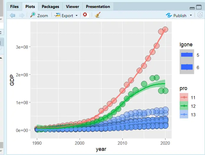
# Set the working environmentsetwd("F:/桌面/R")中国城市数据库 <-readxl::read_excel("中国城市数据库.xlsx")# Load the packageslibrary(ggplot2)library(dplyr)# Rename the dataset columnsnames(中国城市数据库)str(中国城市数据库)data<-rename(中国城市数据库,year= 年份 ,GDP=`地区生产总值(万元)` ,one = `第一产业增加值(万元)` ,id=`行政区划代码`)data<-mutate(data,pro=substr(id,1,2),# Extract characters; the first two digits of cityid represent the provincelgone=log(one,base=10)# Log-transform)# Plotp<-ggplot(data[1:400,],mapping=aes(x=year,y=GDP,size=lgone,# Bubble size weightcolor=pro,# Line color grouping, by provincefill=pro))# Fill color grouping, by provincep+geom_point(shape=21,colour="black",alpha=.5)+geom_smooth(method="loess",aes(group=pro))
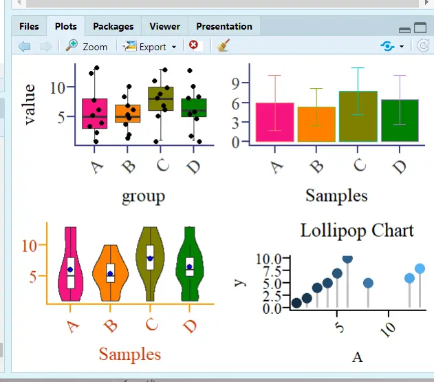
# cowplot packagecowplot::plot_grid(p1,p2,p3,p4,ncol=4)# gridExtra packagegridExtra::grid.arrange(p1,p2,p3,p4,layout_matrix=rbind(c(1,2),c(3,4)))# Split the figure into 4 regions; the top two hold Figure 1 and Figure 2, and the bottom two hold Figure 3 and Figure 4gridExtra::grid.arrange(p1,p2,p3,p4,layout_matrix=rbind(c(1,2,3,4)))# Arrange horizontallygridExtra::grid.arrange(p1,p2,p3,p4,layout_matrix=rbind(c(1),c(2),c(3),c(4)))# Arrange vertically
A 2x2 split
Econometrics
Recommended package: the bruceR package developed by Zhihu expert 包寒吴霜, with the goal of replacing SPSS! I often read this expert’s articles on regression, and in their view, economic regression is just a special variant of general/generalized/multilevel linear models.
Since R is mainly used in biomedical statistics, the mainstream R package three-line tables and the three-line tables required in economics are not the same.
Descriptive Statistics and Output
Descriptive Statistics
1
2
3
4
5
6
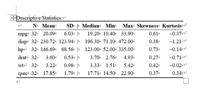
library(bruceR)head(mtcars)# Data bundled with Rmtcarsdemo<-mtcars[c("mpg","disp","hp","drat","wt","qsec")]Describe(mtcarsdemo,digits=2,file="describe")# digits means the number of decimal places to keep# Output the result to Word
Output result
Correlation Analysis
The package this expert developed is terrifyingly good! Short, elegant, and efficient!
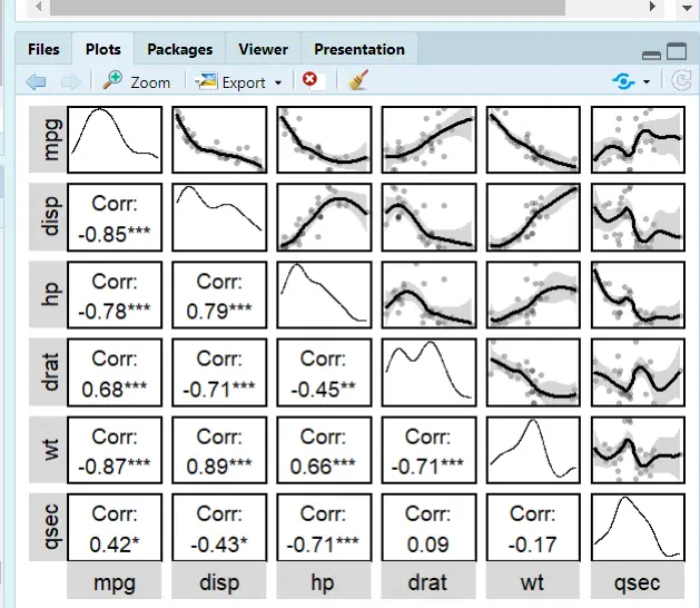
Still using the Describe command
1
2
3
4
5
6
7
library(bruceR)Describe(mtcarsdemo,# Datasetdigits=2,# Decimal placesplot=T,# Plotting featureupper.triangle=T,# Scatter plots in the upper-right triangleupper.smooth="loess")# Fitted line; lm is linear, loess is quadratic
bruceR’s correlation analysis; I was stunned the first time I used it!
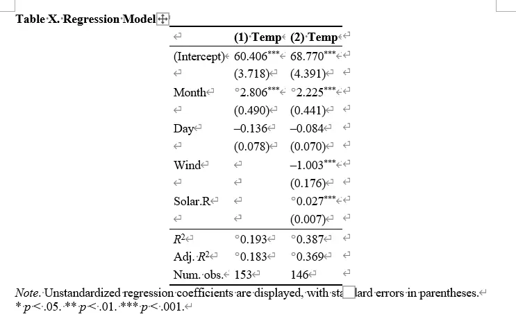
Regression and Word Output
Regression
robust="HC1": robust mode setting; HC1 is reg y x,r in Stata
cluster="stratum": same as Stata; cluster is hierarchical clustering to handle autocorrelation
family=binomial: whether to use binomial regression

 滑翔闪 included in Software Tools and Learning R