I am recording these study notes because of the elegance of the calculus of variations. The reference book is “Fundamentals of Dynamic Optimization” by Alpha C. Chiang, which is a very friendly introductory textbook on dynamic optimization for economics students.
These notes are based on my quick study and personal understanding. If there are any inaccuracies, please bear with me.
Functional
Let’s start with the study of functions.
In elementary school, we began to encounter unknowns like $x$.
In middle school, we started to learn about specific functions like $f(x) = ax + bx^2 + c$.
In high school, we began to understand abstract functions like $f(x) = f(-x)$ and $f’(x) = f(x)$.
In university, we started to learn about implicit functions like $y’ = y + y’’$, which solve a class of functions.
As our study of functions moves from concrete to abstract, we begin to develop the ability to infer the form of a function based on its properties.
Nonlinear functionals in functional analysis are functions of functions. Given specific functional characteristics, we can narrow down the range of functional forms and then select the optimal function based on constraints.
For example, a firm choosing the optimal production process, or an architect selecting the best curve for a building…
Previously, given a specific type of function, we sought extremum points;
Now, given functional characteristics, we seek the best specific function.
Generally, the characteristic constraints of a function can be expressed as $f(t, y(t), y’(t))$, which can be understood as $f(\text{time}, \text{state}, \text{direction})$.
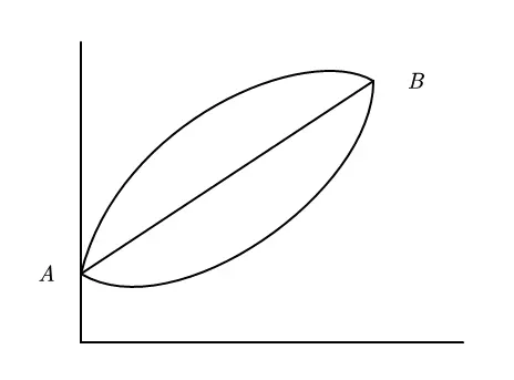
As shown in the figure below, there are three functions from $a$ to $b$ that satisfy the functional characteristics. Which one is the optimal? This introduces the use of calculus to find the extremum of the functional path.
Functions satisfying constraints
$$
V(t) = \int_0^T f(t, y, y’) dt
$$
As the functional form $y$ changes, $V(t)$ also changes. This is the starting point of functional analysis. We aim to find the optimal path $y^*$ from a set of functional forms $y$ by seeking the extremum of $V(t)$ and other constraints.
Calculus of Variations
When learning about derivatives, we used the concept of approximation to find limits:
$$
\lim_{\Delta x \rightarrow 0} \frac{f(x + \Delta x) - f(x)}{\Delta x}
$$
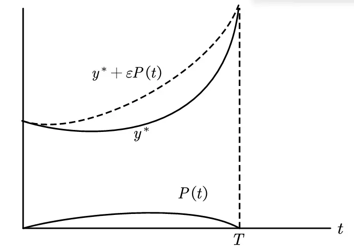
Here, we use a similar approach. Assume the optimal function is $y^*$, and represent a class of functions near it as $y^* + \varepsilon P(t)$ .
Note that $P(0) = P(T) = 0$
Functional representation
Thus, we obtain the following expression in terms of $\varepsilon$:
$$
V(\varepsilon) = \int_0^T F\left[t, \underbrace{y^*(t) + \varepsilon p(t)}_{y(t)}, \underbrace{y^*(t) + \varepsilon p’(t)}_{y’(t)}\right] dt
$$
The first-order condition for the extremum is $\frac{dV}{d\varepsilon} = 0$.
Next, we transform the $\color{red}{\text{red part}}$ using integration by parts $\int_{t=a}^{t=b} v du = vu \big|_{t=a}^{t=b} - \int_{t=a}^{t=b} u dv$ (where $u = u(t)$, $v = v(t)$):
$$
\begin{align}
& \color{red}{\int_0^T F_{y’} p’(t) dt} \\
&= \left[ F_{y’} p(t) \right]_0^T - \int_0^T p(t) \frac{d}{dt} F_{y’} dt \\
&= -\int_0^T p(t) \frac{d}{dt} F_{y’} dt \\
& (\text{Because } P(0) = P(T) = 0\\
& \text{ see the image of the perturbation function } P(t))
\end{align}
$$
Substituting the $\color{red}{\text{red part}}$ back, we get:
$$
\int_0^T p(t) \left[ F_y - \frac{d}{dt} F_{y’} \right] dt = 0
$$
Considering that the perturbation function $P(t)$ can be any function, the only way for the above equation to be zero is if $F_y - \frac{d}{dt} F_{y’} = 0$.
Thus, we obtain the Euler equation:
$$
F_y - \frac{d}{dt} F_{y’} = 0, \quad t \in [0, T]
$$
When the equation constraint only involves three variables, i.e., $F(t, y, y’)$, it can be expanded as:
$$
\begin{aligned}
\frac{dF_{y’}}{dt} &= \frac{\partial F_{y’}}{\partial t} + \frac{\partial F_{y’}}{\partial y} \frac{dy}{dt} + \frac{\partial F_{y’}}{\partial y’} \frac{dy’}{dt} \\
&= F_{ty’} + F_{yy’} y’(t) + F_{y’y’} y’’(t)
\end{aligned}
$$
Expanding, we get:
$$
F_{y’y’} y’’(t) + F_{yy’} y’(t) + F_{ty’} - F_y = 0, \quad t \in [0, T]
$$
A problem
Given the functional $V(y) = \int_0^2 (12ty + y’^2) dt$
The general solution to the Euler equation is $y^*(t) = t^3 + c_1 t + c_2$
Extensions of the Euler equation
Here, we only mention the extensions without further elaboration.
When the functional $F$ contains only some variables, such as $F(t, y’)$, $F(y, y’)$, or $F(t, y)$, there are shortcut methods for each case.
The core of the Euler equation is $F_y - \frac{d}{dt} F_{y’} = 0, \quad t \in [0, T]$
When the functional $F$ contains multiple variables or higher-order variables, the core remains the same, but further expansion is needed.
The Catenary Problem
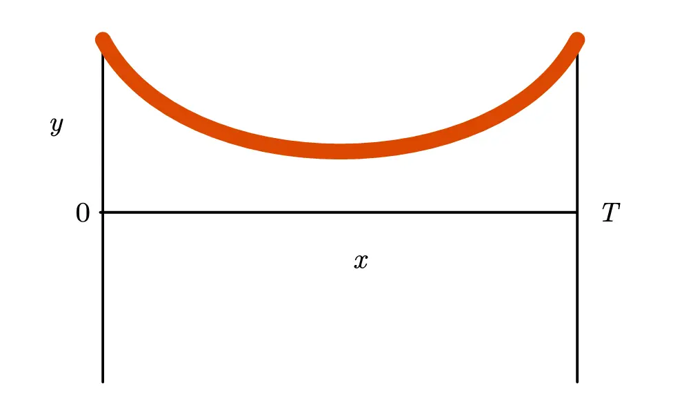
Imagine a red string hanging between two poles for drying clothes.
Establish a coordinate system and rotate this string around the x-axis. What curvature should the string have to minimize the surface area of the resulting solid?
Even a humble clothesline has profound principles
Consider the Pythagorean theorem for a differential element:
$$
(ds)^2 = (dx)^2 + (dy)^2
$$
We can obtain the differential of the curve:
$$
\frac{ds}{dt} = \sqrt{1 + \left( \frac{dy}{dt} \right)^2} = (1 + y’^2)^{1/2}
$$
By differentiating along the curve, the integral of the circumference of each differential circle ($2\pi r$) gives the surface area after rotation.
Thus, we obtain the following functional:
$$
V(t) = \int_0^T 2\pi y ds = 2\pi \int_0^T y (1 + y’^2)^{1/2} dt
$$
Simplifying the expression:
$$
V(t) = \int_0^T y (1 + y’^2)^{1/2} dt
$$
Using the Euler equation, we get:
$$
y (1 + y’^2)^{1/2} - y y’^2 (1 + y’^2)^{-1/2} = c
$$
Simplifying (by rationalizing the denominator and squaring to eliminate the square root in the denominator), we obtain:
$$
y’ \left( \equiv \frac{dy}{dt} \right) = \frac{1}{c} \sqrt{y^2 - c^2}
$$
Which is:
$$
\frac{c dy}{\sqrt{y^2 - c^2}} = dt
$$
Integrating, we get:
$$
\int \frac{c dy}{\sqrt{y^2 - c^2}} = c \ln \left( \frac{y + \sqrt{y^2 - c^2}}{c} \right) + c_1 = \int dt = t + c_2
$$
Rearranging the above expression and combining the two arbitrary constants $c_1$ and $c_2$ into $k$, we obtain the general solution:
$$
y^*(t) = \frac{c}{2} \left[ e^{(t + k)/c} + e^{-(t + k)/c} \right]
$$
And the catenary curve is of the form:
$$
y = \frac{1}{2} (e^t + e^{-t})
$$
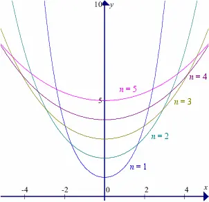
Catenary curve, image from Wikipedia
A uniformly dense string (e.g., a clothesline) hanging under uniform gravitational force will also form this curve.
Suspension bridges, hyperbolic arch bridges, and overhead cables all utilize the principles of the catenary curve.
In architectural design, the following form is generally used:
$$
y = c + a \cosh \frac{x}{a}
$$
Nature and society are always under optimal control!
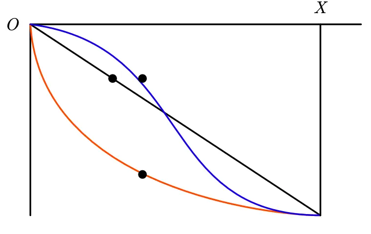
The Brachistochrone Problem
Imagine a marble race with three different slides. A contestant has only one chance to choose. Which slide should they choose for the marble to reach the finish line the fastest?
Yes, even slides hide profound principles
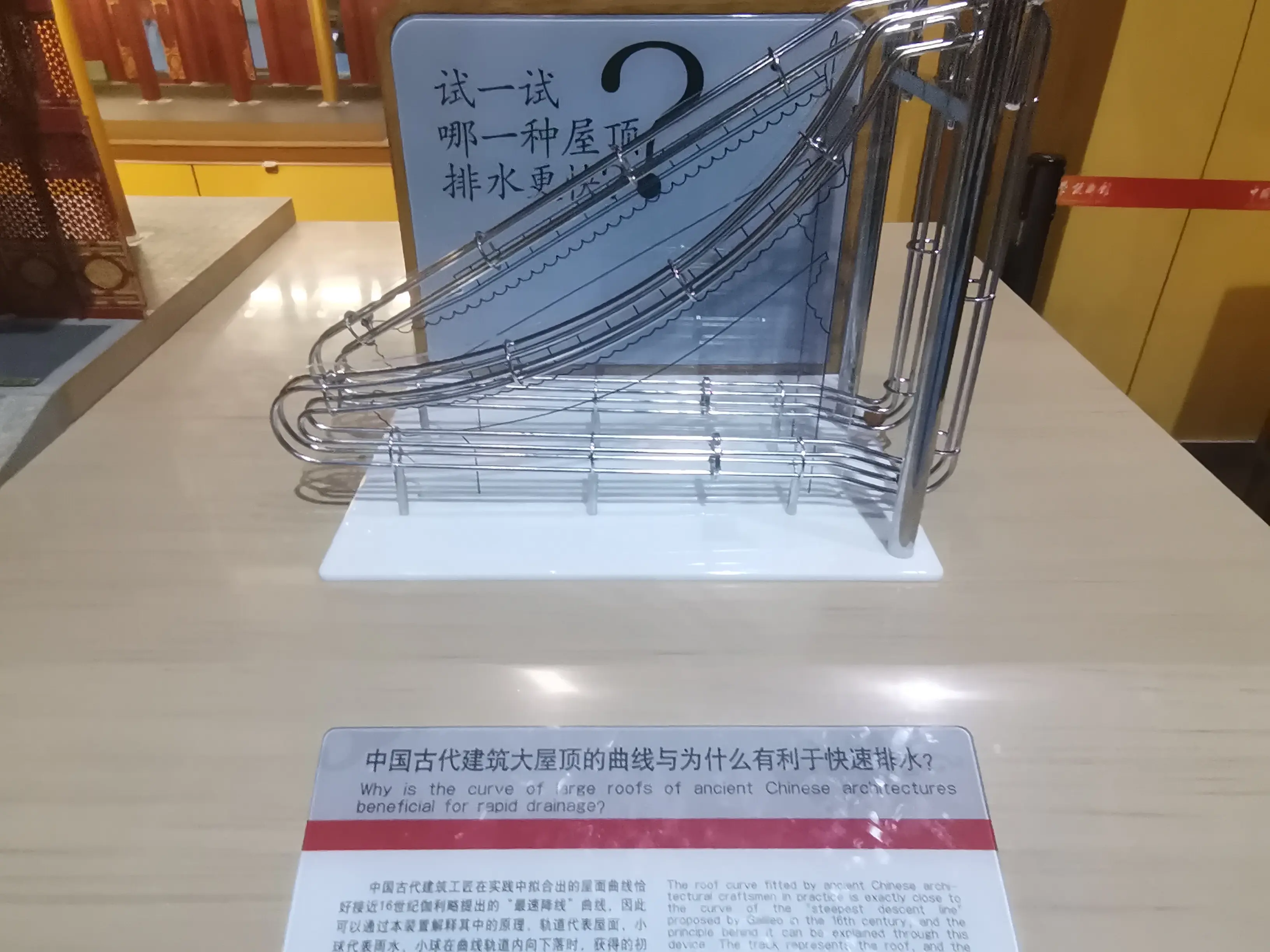
Source: Beijing Science and Technology Museum. Imagine ancient architecture; which building curve would facilitate easier drainage? The logic is the same.
Using the conservation of energy, we get:
$$
\begin{align}
\frac{1}{2} m v^2 &= m g y \
v &= \sqrt{2 g y}
\end{align}
$$
In the catenary problem, we introduced the differential of the curve as $ds = (1 + y’^2)^{1/2} dt$.
Thus, considering velocity as the derivative of distance with respect to time:
$$
v = \frac{ds}{dt} = \sqrt{1 + y’^2} \frac{dx}{dt}
$$
Combining the above equations:
$$
\begin{cases}
v = \sqrt{2 g y} \
v = \sqrt{1 + y’^2} \frac{dx}{dt}
\end{cases}
$$
We obtain:
$$
dt = \frac{\sqrt{1 + y’^2}}{\sqrt{2 g y}} dx
$$
The target functional seeks the minimum total time:
$$
T = \int dt = \int \frac{\sqrt{1 + y’^2}}{\sqrt{2 g y}} dx
$$
Using the Euler equation, we get:
$$
2 y’’ y + y’^2 + 1 = 0
$$
For the complete solution, refer to A Brief Discussion on the Calculus of Variations, which also mentions other mathematicians’ solutions to this problem.
In any case, one form of the solution is (where $a$ and $c$ are arbitrary constants):
$$
\begin{cases}
x = a (\theta - \sin \theta) + c \
y = a (1 - \cos \theta)
\end{cases}
$$
This form is related to the cycloid.
Source: Wikipedia
Monopoly Economics Problem
Consider a monopoly firm with a profit function written as $F(P, P’)$.
The economic meaning is that the monopoly firm has the power to set prices.
The functional is then:
$$
V = \int F(P, P’) dt
$$
Substituting into the Euler equation, we get:
$$
F_{P’P’} P’’ + F_{PP’} P’ - F_P = 0
$$
Solving this implicit function requires some clever manipulation. Multiply both sides by $P’$ and then rearrange:
$$
\begin{aligned}
& \frac{d}{dt} (P’ F_{P’} - F) \\
& = \frac{d}{dt} (P’ F_{P’}) - \frac{d}{dt} F(P, P’) \\
& = F_{P’} P’’ + P’ \left( F_{PP’} P’ + F_{P’P’} P’’ \right) - \left( F_P P’ + F_{P’} P’’ \right) \\
& = P’ \color{red}{\left( F_{P’P’} P’’ + F_{PP’} P’ - F_P \right)}
\end{aligned}
$$
The red part is the original equation.
Thus, we obtain:
$$
F - P’ F_{P’} = c
$$
Where $c$ is a constant. Writing $F$ as the common profit function $\pi$, we get:
$$
\pi - P’ \frac{\partial \pi}{\partial P’} = c
$$
Considering static monopoly, the monopoly firm makes only one pricing decision (more detailed static game theory also considers product differentiation, information asymmetry, game sequence, and firm entry/exit states).
In this case, the profit function only depends on $P$ and not on $P’$ (since there is only one pricing decision, no price change occurs). Clearly, $P’ \frac{\partial \pi}{\partial P’} = 0$, so $\pi_s = c$.
Now, consider dynamic game theory on top of static game theory. After the first pricing decision, monopoly firms begin to make multiple pricing decisions. The profit function is now:
$$
\pi - P’ \frac{\partial \pi}{\partial P’} = \pi_s
$$
Here, the profit function $\pi$ must depend on both $P$ and $P’$. Thus, consider the elasticity of $\pi$ with respect to $P’$, denoted as:
$$
\frac{\partial \pi}{\partial P’} \frac{P’}{\pi} = \varepsilon_{\pi P’}
$$
Substituting into the dynamic monopoly game formula, we get:
$$
\varepsilon_{\pi P’} = 1 - \frac{\pi_\varepsilon}{\pi}
$$
In other words, in dynamic monopoly, firms should continuously adjust their profit functions based on this relationship.