1. What are the causal frameworks?

Today, with numerous causal frameworks emerging and various disciplines such as statistics (including pharmacology and psychology, each with its own statistical interpretation), economics, and computer science having their own schools of thought, the landscape has become intricate and diverse. It is intertwined and complex, and I am not entirely sure about the overall system.

Personally, I have been exposed to Judea Pearl’s Structural Causal Model (SCM) the most. Regarding his work “The Book of Why,”¹ My personal understanding is that association-intervention-counterfactual represents the three levels of causality. The selection of control variables controls for backdoor paths, while setting instrumental variables controls for frontdoor paths.

The knowledge about ATE (Average Treatment Effect), ATT (Average Treatment Effect for the Treated), ITT (Intention-to-Treat), and LATE (Local Average Treatment Effect) appears sporadically in “Mostly Harmless Econometrics” ¹. The entire framework is based on Donald Rubin’s proposal of the Potential Outcome Framework (also known as Rubin Causal Model, abbreviated as RCM).

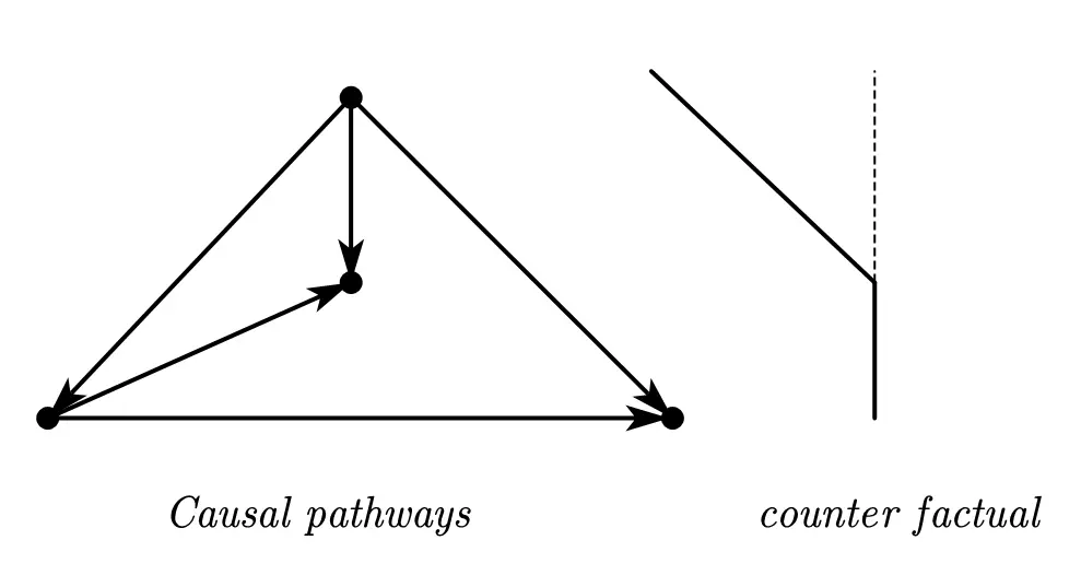
It’s interesting that Judea Pearl (in “The Book of Why”) proposes that counterfactuals under causal pathways are the same as Rubin’s concept of “potential outcomes.” However, Rubin responded that the two are completely different ²and does not endorse the analysis method of path diagrams. (Personally, I find it difficult to understand Rubin’s response, as in my view, the direction of arrows in SCM corresponds to the direction of addition and subtraction signs in RCM).

As far as I know, causal analysis in statistics is currently divided into frequentist and Bayesian schools of thought. Research is conducted to understand causal inference through Markov chains. Personally, I am quite unfamiliar with this area of knowledge. My understanding of this topic mainly comes from educational videos by Fmajor on Bilibili.

2. More details about RCM

ATE (Average Treatment Effect), ATT (Average Treatment Effect for the Treated), ITT (Intention-to-Treat), and LATE (Local Average Treatment Effect) are different statistical estimators.

From ATE to ATT

Starting from elementary school, we have been exposed to comparing and analyzing data using the mean of various groups. However, this type of group comparison is just the starting point for causal discussions. It is necessary to further decompose these group differences to explore causal relationships.

Average Treatment Effect (ATE): The difference between the means of two groups is directly used as the estimator. It can be considered as the difference between the population means or as the mean difference between groups (e.g., in the estimation of twin data):

$$\bar Y_1-\bar Y_0=\sum_{i=1}^{N}\frac{Y_{i}(1)-Y_{i}(0)}{N}$$

Treating $D_i$ as the treatment variable, where $D_i = 1$ represents the experimental group and $D_i = 0$ represents the control group, the linear equation is as follows:

$$\begin{align}Y_{i}&=\begin{cases} Y_{1i} \quad if D_i = 1 \newline Y_{0i} \quad if D_i = 0 \end{cases} \newline &=Y_{0i}+(Y_{1i}-Y_{0i})D_{i} \end{align}$$

Subtracting the two equations, we obtain the following expression:

$$\begin{aligned} &\mathbf{E}[Y_{i}\mid D_{i}=1]-\mathbf{E}[Y_{i}\mid D_{i}=0]\newline& =\color{red}{\underbrace{\mathbf{E}\lfloor Y_{1i}\mid D_{i}=1\rfloor-\mathbf{E}[Y_{0i}\mid D_{i}=1]}_{\text{ATT}} } \newline &+\underbrace{\mathbf{E}[Y_{0i}\mid D_{i}=1]-\mathbf{E}[Y_{0i}\mid D_{i}=0]}_{SelectionBias} \end{aligned}$$

Where $\mathbf{E}[Y_{0i}\mid D_{i}=1]$ is intentionally introduced by us, representing another “parallel universe” that we wish to explore but cannot directly observe—assuming that the subgroup represented by $\mathbf{E}[Y_{\color{blue}{1i}}\mid D_{i}=1]$ did not receive the treatment in the parallel world. Their state is denoted as $\mathbf{E}[Y_{\color{blue}{0i}}\mid D_{i}=1]$, which is the “potential outcome” that Rubin aims to find.

$\color{red}{\mathbf{E}\left[ Y_{1i}\mid D_{i}=1 \right] - \mathbf{E}[Y_{0i}\mid D_{i}=1]}$ represents the Average Treatment Effect on Treated (ATT). There is no better controlled experiment than “a binary choice splitting into two parallel universes”, but no one can truly obtain such data! Therefore, economists attempt to estimate ATT through ATE, hence the introduction of randomized controlled trials (RCTs).

RCT: Making ATE approach ATT

RCT stands for Randomized Controlled Trial, representing a randomized experiment. Under the conditions of a randomized experiment, ATE = ATT. Next, let’s delve into the explanation:

Subtracting the subgroup $\mathbf{E}[Y_{0i}\mid D_{i}=1]$ from the subgroup that has never received treatment in the real world $\mathbf{E}[Y_{0i}\mid D_{i}=0]$, if the result is non-zero, selection bias occurs.

The reason may be sampling selection bias: for example, conducting a fitness-related survey only at gyms would definitely not achieve effective comparison; another example is the well-known survivorship bias in the military, where the returned planes are the ones that survived, making it unreliable to estimate the areas that need reinforcement based on their damages.

It could also be self-selection bias: for example, an uneven gender ratio in admissions does not necessarily indicate discrimination, as this analysis overlooks the gender ratio in application tendencies. Some genders may be more inclined to apply for more challenging positions, leading to higher rejection rates; police enforcement focusing more on a certain race does not necessarily imply discrimination, as it may simply reflect higher crime rates within that race.

Omitted variables, model errors, measurement errors, and insufficient sample size can all contribute to bias.

If we use the method of randomized trials, the samples are randomly distributed. We hope that this randomized trial can average out some unobserved influencing variables, thereby making $D_i$ and $Y_{0i}$ independent, which means $\mathbf{E}[Y_{0i}\mid D_{i}=1]=\mathbf{E}[Y_{0i}\mid D_{i}=0]=\mathbf{E}[Y_{0i}]$.

At this point, the estimation of ATE has been effectively simplified:

$$\begin{aligned} &\mathbf{E}[Y_{1i}\mid D_{i}=1]-\mathbf{E}[Y_{0i}\mid D_{i}=1]\newline&=ATT =\mathbf{E}[\mathbf{Y}_{1i}-\mathbf{Y}_{0i}\mid D_{i}=1] \newline &=ATE=\mathbf{E}[Y_{1i}-Y_{0i}] \end{aligned}$$

Further estimating through regression equations:

$$\begin{align}Y_{i}&=\begin{cases} Y_{1i} \quad if D_i = 1 \newline Y_{0i} \quad if D_i = 0 \end{cases} \newline &=Y_{0i}+(Y_{1i}-Y_{0i})D_{i} \newline & =\alpha+\rho D_i+\eta_i \end{align}$$

$$\begin{aligned}&\operatorname{\mathbf{E}}[Y_i\mid D_i=1]=\alpha+\rho+\operatorname{\mathbf{E}}[\eta_i\mid D_i=1]\newline &\operatorname{\mathbf{E}}[Y_i\mid D_i=0]=\alpha+\operatorname{\mathbf{E}}[\eta_i\mid D_i=0]\end{aligned}$$

We can obtain the difference between the two.

$$\begin{aligned}&\operatorname{\mathbf{E}}[Y_i\mid D_i=1]-\operatorname{\mathbf{E}}[Y_i\mid D_i=0]\newline &=\underbrace{\rho}_\text{Treatment effect}+\underbrace{\operatorname{\mathbf{E}}[\eta_i\mid D_i=1]-\operatorname{\mathbf{E}}[\eta_i\mid D_i=0]}_\text{secletion bias}\end{aligned}$$

When there is selection bias $\eta_i \neq 0$, it means that the residual is correlated with $D_i$. We emphasize randomized trials because we hope that random intervention experiments can make the two unrelated, eliminating this selection bias. So when randomized trials are satisfied, $\eta_i=0$, $ATE \xrightarrow{RCT} ATT$.

This also tells us why we should pay attention to residual analysis.

From ITT to LATE

Intention to Treat (ITT). Although randomized intervention trials are useful, the variables we want to study are not always randomly distributed. For example, industrial land tends to aggregate around certain grades of land. In this case, buyers are not randomly distributed. In such scenarios, we consider other randomly distributed variables that may influence their decisions.

It’s more illustrative to first understand this using the path diagram of SCM:

Angrist (2011) is a paper that examines the impact of participating in the Vietnam War on income. In this study, the variable of military enlistment was found to be problematic, so the author used enlistment eligibility as an instrumental variable. (Nostalgic for the era of short 6-page econometric papers)

Clearly, there exists a process where an individual is first informed of their enlistment eligibility and then decides whether to enter the military.

The ITT equation is as follows:

It can be observed that the ITT estimate is quite similar to $\mathbf{E}[Y_{i}\mid D_{i}=1]-\mathbf{E}[Y_{i}\mid D_{i}=0]$, meaning that when $D_i$ and $Z_i$ are one-to-one corresponding, i.e., when $z=d$, ITT = ATE.

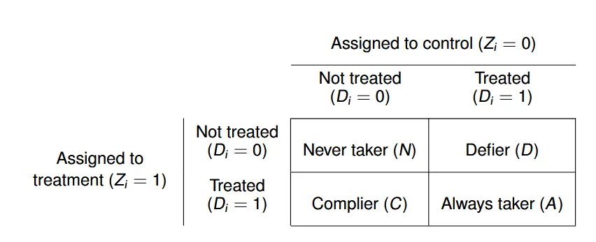
• $\pi_N$: Regardless of whether I am eligible or not, I will never join the military.
• $\pi_D$: Contrarian attitude, I will join the military if I am eligible, and I will refuse if I am not eligible.
• $\pi_A$: Regardless of whether I am eligible or not, I will always join the military.
• $\pi_C$: Compliance, I will join if eligible, and I will not join if not eligible.

Due to the non-random distribution of $Di$, as we are based on a sample of military personnel for statistics, we have only the following equation:

$$\begin{aligned} \mathbf{E}[D_i=1|Z_i=0]=\pi_A+\pi_D\newline \mathbf{E}[D_i=1|Z_i=1]=\pi_A+\pi_C \end{aligned}$$

In this case, we cannot estimate $\pi_i$ separately for $\pi_i$ , $i∈{A,C,D,N}$.

However, due to the random distribution, the results will be proportional, allowing us to derive a linear equation:

The solution is to make an assumption — quite reminiscent of an economics joke. Here’s the original joke:

A physicist, a chemist, and an economist are stranded on a deserted island, starving. Suddenly, a can of food washes ashore. The physicist says, “We can use rocks to apply momentum to the can, causing its surface to fatigue and rupture.” The chemist says, “We can make a fire, then heat the can, causing it to expand until it bursts.” The economist then says, “Let’s assume we have a can opener…”

After introducing the assumption, we directly obtain the LATE:

$$\mathrm{LATE}=\mathrm{CATE}_{\mathcal{C}}=\frac{\mathrm{ITT}}{\pi_{\mathcal{C}}}$$

$$\small \hat{\mathbf{CATE}_C}=\frac{\mathbf{E}\Big[Y_i|Z_i=1\Big]-\mathbf{E}\Big[Y_i|Z_i=0\Big]}{\mathbf{E}\Big[D_i|Z_i=1\Big]-\mathbf{E}\Big[D_i|Z_i=0\Big]}=\frac{\mathrm{effect~of~}Z_i\text{ on }Y_i}{\mathrm{effect~of~}Z_i\text{ on }D_i}=\frac{\operatorname{ITT}_Y}{\operatorname{ITT}_D}$$

The LATE section heavily relies on the Oxford course material. For a more algebraic explanation, refer to the Harvard course material and “Mostly Harmless Econometrics.”

Social science attributes in mathematical economics

The social science attributes in mathematical economics are evident in the need to articulate assumptions that capture social phenomena. For instance, when studying unique policies, it’s essential to argue that the policy affects everyone, reflecting the assumption of monotonicity. Similarly, when using instrumental variables, it’s crucial to discuss the social relationship between the instrument and the explanatory variable. These assumptions serve as concise descriptions of social phenomena, highlighting the distinct social science nature of economic analysis.

Recently, as I delve into advanced macroeconomics, I’ve come to realize the methodical nature of this field. The techniques in advanced macroeconomics, such as the variational calculus and Lagrangian method, address optimization in classical models. However, the challenge lies in navigating through the myriad of assumptions and transformations imposed on each macroeconomic model. Whether it’s manipulating formulas or introducing sudden assumptions, the goal is to distill economic phenomena into characteristic features and then formalize them mathematically. This, I believe, is the greatest challenge. Examples include the production function for knowledge (treating knowledge as a factor of production), the Cobb-Douglas production function (exhibiting constant returns to scale), household constraints (consumption discounting being less than wealth discounting), and household utility functions (risk aversion).

In essence, the distinguishing factor between economists with a background in economics and those with a background in mathematics lies in the framework used to explore equilibrium, construct functions that capture economic phenomena, and formulate optimization constraints. This represents the essence of economic thinking and intuition that sets economists apart in the realm of mathematical economics.

As an aside, I’d like to share my notes on advanced macroeconomics.

Summarize

Further examples illustrate that the Difference-in-Differences (DID) estimation is the Average Treatment Effect on the Treated (ATT); the Regression Discontinuity Design (RDD) estimation is the Local Average Treatment Effect (LATE); and the Instrumental Variable (IV) and RDD estimations are the same under certain conditions.

ATT and LATE are what we aim for, longing for a perfect control experiment like the parallel universe, but what we have are only the Average Treatment Effect (ATE) and Intention to Treat (ITT).

When the treatment variable (D) satisfies the Randomized Controlled Trial (RCT), ATE equals ATT.

When D does not satisfy RCT but the instrumental variable (Z) does, and assuming monotonicity and relevance, we can construct IV or RDD, and in this case, ITT equals LATE.

When neither D nor Z satisfies RCT, other methods are used to estimate counterfactual situations, such as cluster analysis (directly estimating the distribution of counterfactuals and contrasting it with the current clustering phenomenon through residual analysis), synthetic control, etc.

Textbooks usually introduce matching theory to achieve these estimation assumptions.

In conclusion, econometric models analyze causal relationships based on such potential outcome frameworks, advocating themselves as causal science.

Seen in this light, doesn’t it embody the magic of “creating something out of nothing” and “inferring causes from effects”?