One-Time Government Investment and Long-Run Industrial Development

This post introduces three papers on one-time government investment and long-run industrial development:

• AER, “Moonshot: Public R&D and Growth”
• QJE, “The Long-Run Impacts of Public Industrial Investment on Local Development and Economic Mobility: Evidence from World War II”
• AER, “America, Jump-Started: World War II R&D and the Takeoff of the US Innovation System”

Government and the market: learn to ask better questions

In debates over industrial policy, the answer depends a great deal on how the question is framed.

1. In the past, we asked it rather crudely: should the government or the market take the lead?
2. Now the question is more precise: between government and market, which one should lead in which domain, and how?

Getting people to agree on a mixed economy was never easy. China and the Soviet Union both went through eras of comprehensive planning, and the United States had its own witch-hunt politics during institutional conflict¹. That, I think, is one reason empiricism became the mainstream². The world is no longer just an ideological fight between all-or-nothing positions. Societies pay a huge price for extreme paths. What we need are sharper boundaries and sharper questions.

All three papers discussed here use World War II-era manufacturing investment as their historical setting. They study the long-run effects of one-time manufacturing investment on manufacturing development. A shared issue running through them is how to distinguish local effects from national effects.

The moonshot shock: public R&D spending and growth

Moonshot: Public R&D and Growth

Introduction

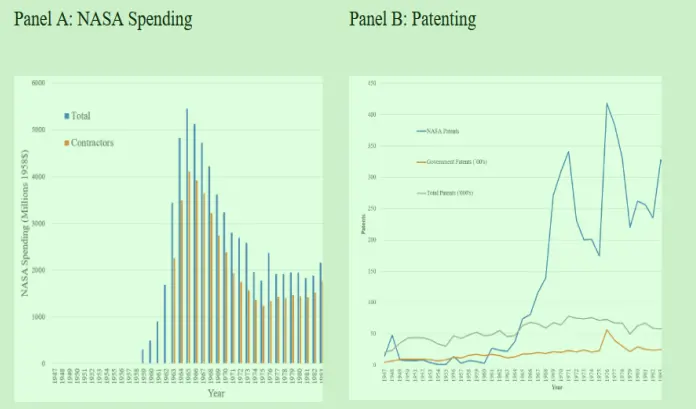
After the Soviet Union launched the first satellite during the Cold War, the United States began investing heavily in the manufacturing side of the space industry.

That historical setting lets us think about several issues:

• How theories of technological progress and economic growth can be tested and extended
• The social return to innovation is larger than the private return, so firms may not have enough incentive to innovate on their own. Does that mean the government needs to provide an extra push?
• Does government stimulus actually work? Can government R&D, or public R&D, generate long-run growth?
• The exogeneity of the event. At the time, NASA investment accounted for 0.7% of US GDP. Geopolitical conflict was an exogenous shock.

Identification strategy

One distinctive feature of Moonshot: Public R&D and Growth is that it makes full use of declassified US materials from the Cold War period.

• Special point 1: the paper uses declassified CIA intelligence files that describe Soviet space capabilities in detail, then matches them with US patents from before Sputnik. That lets the authors use textual similarity to locate where relevant patent technologies had been developing.
• Special point 2: NASA invested directly in firms that already had a patent base, rather than doing the R&D itself from scratch. That is why the paper can estimate the effects by comparing patent data through textual similarity.

Triple difference:

$$ \begin{equation} \begin{aligned} Y_{ijt} = \beta_1 &+ \beta_2 High\_Space\_Capability_{ij<1958} \times SpaceRace_t \\ & + \beta_3 High\_Space\_Capability_{ij<1958} \times Post\_SpaceRace_t \\ & + {\color{red}{\beta_4}} High\_Space\_Capability_{ij<1958} \times SpaceRace \times Space\_Industry_j \\ & + {\color{red}{\beta_5}} High\_Space\_Capability\_{ij<1958} \times Post\_SpaceRace_t \times Space\_Industry_j \\ & + TotalPre\_1958Patents_{ij} \times \gamma_t \\ & + \delta_i + \theta_j + \gamma_t + v_{ijt} \end{aligned} \end{equation} $$

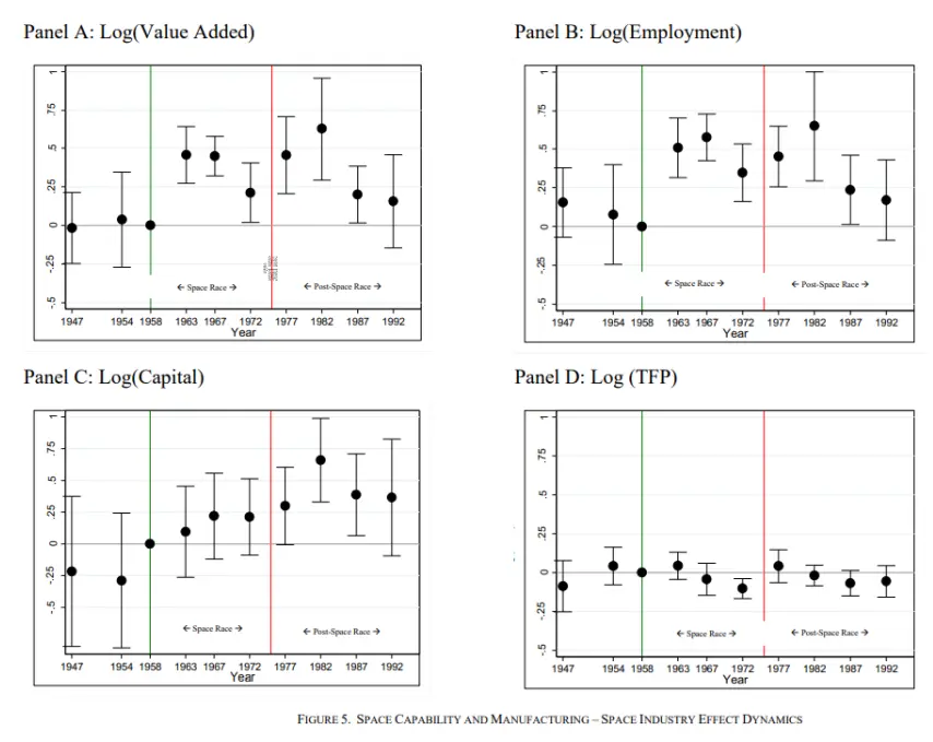
${\color{red}{\beta_4}}$ captures the effect during the investment period. ${\color{red}{\beta_5}}$ captures the long-run effect after the investment ended.

• Y: NASA-related regional investment, patent, and industry outcomes (value added, TFP, employment, capital)
• HighSpaceCapability: patent-text similarity before the race began
• SpaceRace: dummy for the space-race period (1959-1972)
• SpaceIndustry: dummy for whether the industry was NASA-related
• PostSpaceRace: time dummy for the post-race period (after 1972)
• TotalPre_1958Patents: number of patents that already existed before 1958

To quantify the magnitude further, the paper estimates a multiplier effect:

$$ \text{Multiplier}=\frac{\beta_{\text{output}}\times\text{output}}{\beta_{\text{investment}}\times\text{investment}} $$

The paper estimates a multiplier of 0.3, which is lower than both the model estimate and the 0.6-0.8 range reported in other papers. The dynamic increase is not especially large either. The authors explain that growth was very rapid in those years, so the multiplier is probably underestimated. The measure also does not really capture R&D done by universities or by NASA’s own research centers.

In econometric work, we usually prefer identification strategies that are more likely to understate the effect. If the real-world effect ends up being larger than what we estimate, that only makes the conclusion more convincing.

Research also shows that instrumental variables can easily magnify estimates, so IV is always a tradeoff between endogeneity and validity.

Robustness

• Tighten the definition of the space industry and add more related industries
• Adjust industry-level standard errors based on NASA shares
• Drop one state or one industry at a time and check how the results change
• Use growth rates rather than productivity as the explained variable
• Instrumental variable: whether an industry-county pair received funding in year t
• Measure NASA spending more precisely and compare the US with non-US cases
• Use non-space samples for cross-industry analysis
• Match patent similarity using US policy documents
• Compare different text-similarity measures

Mechanism tests

The main results ask whether time-specific investment persisted over time. The mechanism section turns to space-specific spillovers. Does industrial development spill over?

Population channel: industrial development attracted in-migration. Using triple differences on panel data of population flows, the paper finds an in-migration effect.

Goods channel: when industry develops, does demand for goods rise as well? The paper translates this into changes in comparative trade advantage, using the quantified comparative-advantage score from Railroads and American Economic Growth: A “Market Access” Approach as the explanatory variable in a triple-difference setup. The result is not significant.

Distinguishing local effects and national effects

Government investment can be seen as a structured allocation of resources. When one region develops, is it creating new value, or is it simply piling up resources and producing distributive inequality? That is worth debating.

A lot of Chinese work, for example, asks whether provincial capitals create a siphoning effect or a blood-making effect. That is the difference between local effects and national effects. The issue also comes up in Fu Peng’s recent talk, which mentions the illusion of government investment:

When the government points resources somewhere, that place develops. It looks like capable government action, but once the government leaves, the investment leaves too. Prosperity of this point-and-shoot kind is structural redistribution, not the creation of wealth. (My paraphrase.)

If we want to see through that illusion in research, we have to widen the lens and distinguish local effects from national effects across a longer span of time and space..

Xiangzhang Economics once discussed an earlier version from two years ago of Moonshot: Public R&D and Growth. That version originally used the arcsinh transformation and difference-in-differences to handle the variables, and it did not discuss the goods channel.

• The shift away from arcsinh and DiD was probably influenced by Logs with Zeros? Some Problems and Solutions, which seems to have pushed the paper toward a different estimation strategy.
• The goods channel was probably added because reviewers criticized the paper for not addressing the identification of local effects and national effects.

The long-run economic payoff of wartime factory construction

The Long-Run Impacts of Public Industrial Investment on Local Development and Economic Mobility: Evidence from World War II

Introduction

This paper studies the persistent effects of World War II manufacturing investment from the perspective of labor economics.

• Phenomenon: children born in places that received wartime plants earn higher wages later in life.
• Debate: what explains that wage gain?
• Possibilities: exposure effects: children grew up in a better environment; welfare effects: local jobs offered better compensation; human capital investment: children developed better skills.

Identification strategy

A few comparison exercises:

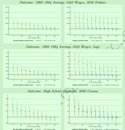
• Wages still rise even when skill levels are held constant.
• Children born locally do not see a clear wage gain if they move away, but they do if they stay.
• Children who move into the area see a clear wage gain relative to those who do not.
• When wage growth is decomposed using education as an explanatory variable, the explained effect is quite small.

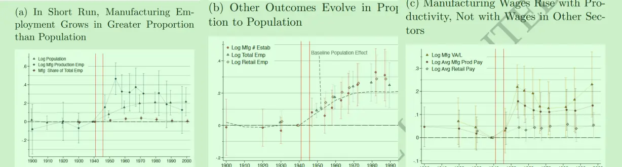
• Counties with large public plants had 30% more manufacturing employment than control counties, 20% more population, and median household income 7-8% higher than the controls.
• Manufacturing employment in treated counties expanded sharply, far outpacing overall population growth.
• Manufacturing employment as a share of total employment increased and remained high throughout the 1970s.
• In the decades after the war, population growth in treated counties kept exceeding that of control areas, eventually stabilizing at a new permanent level roughly 20% above the controls.
• The number of firms did not increase. What increased was scale.

Taken together, the wage growth seems to come from welfare effects.

Distinguishing local effects and national effects

What if World War II had never happened? Without the war, the country would obviously have built plants in economically developed areas. So wartime rear-area plant construction should have different effects from plants that would have been built endogenously in already-developed places.

The paper checks this with contemporary Million Dollar Plants data and finds that this wage effect disappears for modern factories.

That leads to the authors’ final discussion: the way plant construction improved local transportation conditions may be the key to the effect.

Because the modern transportation system is already well developed nationwide, the welfare effect has weakened.

America jump-started: World War II R&D and the innovation system

America, Jump-Started: World War II R&D and the Takeoff of the US Innovation System

Introduction

How the US innovation network took shape is still an important question.

As an aside, I personally lean toward the view that talent immigration was a major reason for US development.

During World War II, the US Office of Scientific Research and Development (OSRD) supported one of the largest public investments in applied R&D in American history. Using data on all OSRD-funded inventions, this paper shows the far-reaching impact of that shock on the US innovation system. It generated technology clusters across the country and increased high-tech entrepreneurship and employment.

Those effects lasted at least into the 1970s, driven mainly by agglomeration forces and endogenous growth. Beyond creating technology clusters, wartime R&D permanently changed the overall trajectory of US innovation, pushing it toward the technological directions funded by the OSRD.

Identification strategy

$$ \ln(Patents)_{ict}=\sum_{t=1931}^{1970}\beta_t\cdot\ln(OSRDrate)_{ic}\cdot Year_t+\alpha_{ic}+\delta_t+\varepsilon_{ict} $$

i is county, c is patent class, and t is year. Standard errors are clustered at the county level. OSRDrate: the share of patent applications in a given class between 1941 and 1948 that were funded by the OSRD.

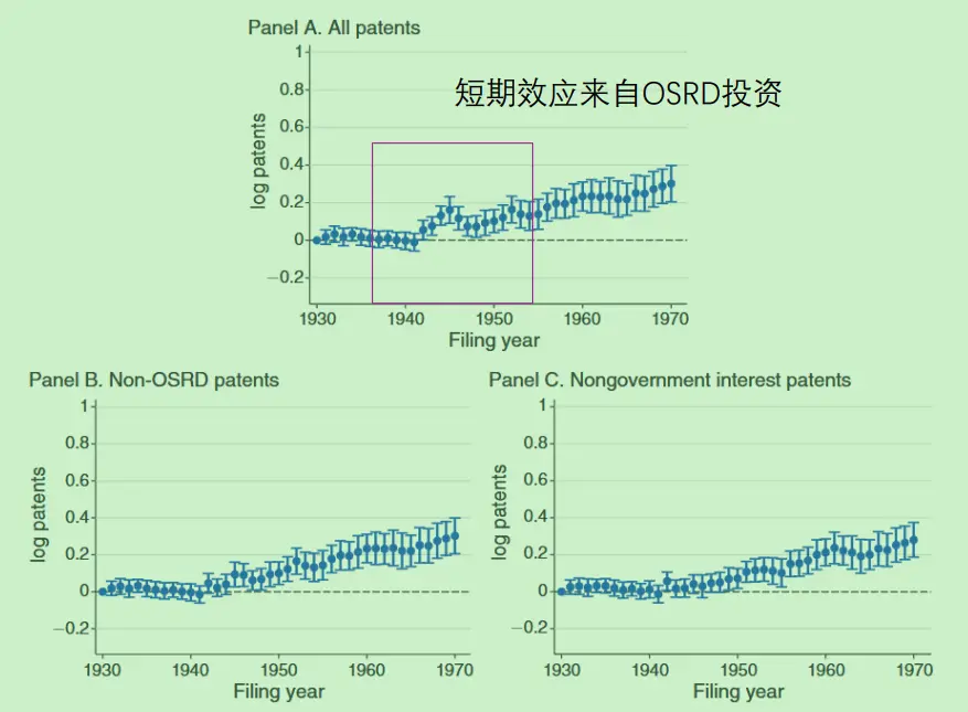
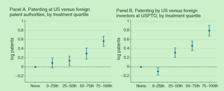
Quantile regression and event-study analysis:

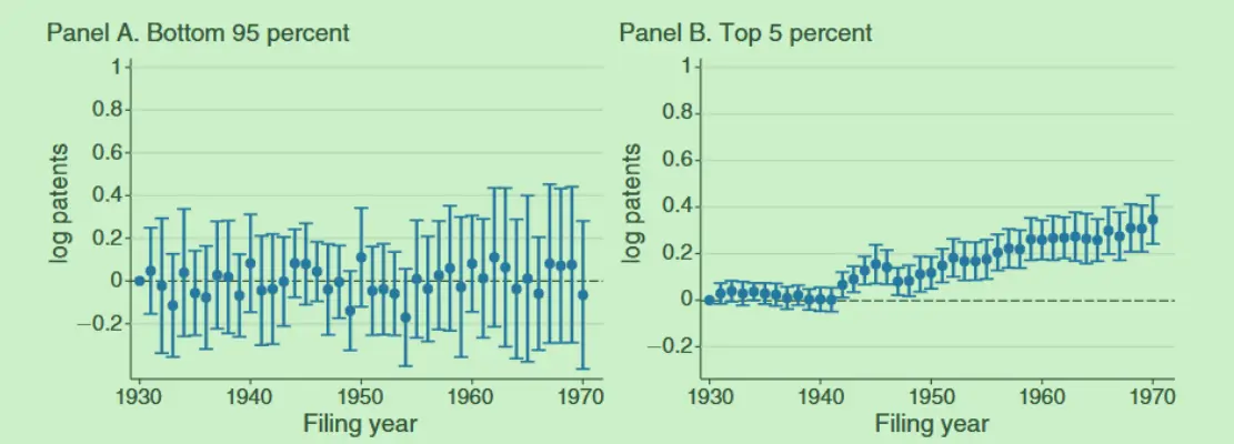
The gap between the top 5% and bottom 5% of OSRD investment is large in both the short run and the long run. The strongest effects appear in electronics and electrical technologies, which were also the patent classes most closely tied to the war.

Mechanism

Patent data contain information on industry, location, citation relationships, and time.

Industries can also be divided into different types and into upstream and downstream positions.

By combining these variables, we can study the formation, expansion, and spillovers of patent networks.

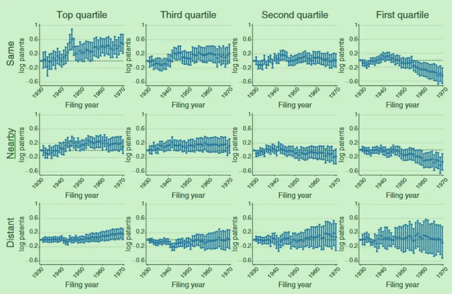
• Quantile regressions within the same county.
• From left to right are investment-rate quantiles.
• From top to bottom, the patent classes become increasingly distant.

The paper has much more to discuss, but I will just sketch a few ideas here:

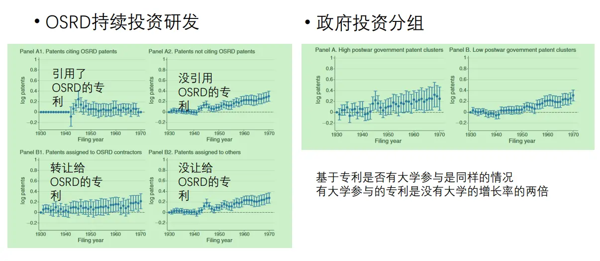
• whether the patent had government involvement
• citation direction: patents citing others and being cited, plus upstream-downstream industry relations
• geographic space: different industries within the same county; the same industry across different counties……
• firms as a whole: all firm patents, firms with patents in the same county and technological field, firms with patents only in different counties and/or technological fields, and firms with no patents.

Distinguishing national effects and local effects

The paper separates the two by comparing the United States, the United Kingdom, and France.

$$ \begin{aligned} \ln(Patents)_{ict} = & \sum_{q=1}^4 \beta_q \cdot 1\{Country_i = US\} \cdot 1\{Class_c \in \text{quartile } q\} \cdot 1 \{t > 1945 \} \\ & + Country_i \times Class_c \\ & + Country_i \times Post_t \\ & + Class_c \times Post_t \\ & + \varepsilon_{ict} \end{aligned} $$

How to present papers

Under my advisor’s guidance, I came to understand that a reading-group presentation should summarize multiple papers around a common theme.

Using this post as an example:

• State the central theme clearly: the common thread across these three papers is one-time government investment and long-run development. In the end, the extra point to watch is the distinction between national effects and local effects. Do not present one paper after another like a running ledger.
• Choose the level of detail well: spend more time sharing the identification strategy, the innovations, and the logic behind the mechanism design. Robustness checks can be covered briefly.
• Keep a learner’s mindset: while presenting, think about what we as learners can actually do with the paper: where it falls short, what is worth learning from, and what is worth imitating……
• Learn how to speak: if you find this line of papers interesting, think about how to structure the presentation so the interesting parts show up quickly.

In collaborations, the part senior scholars abroad often write themselves is the introduction. That is exactly where this ability shows up.